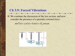
Ch 3.9: Forced Vibrations
Ch 3.9: Forced Vibrations. We continue the discussion of the last section, and now consider the presence of a periodic external force:. Forced Vibrations with Damping. Consider the equation below for damped motion and external forcing funcion F 0 cos t .

Ch 3.9: Forced Vibrations
E N D
Presentation Transcript
Ch 3.9: Forced Vibrations • We continue the discussion of the last section, and now consider the presence of a periodic external force:
Forced Vibrations with Damping • Consider the equation below for damped motion and external forcing funcion F0cost. • The general solution of this equation has the form where the general solution of the homogeneous equation is and the particular solution of the nonhomogeneous equation is
Homogeneous Solution • The homogeneous solutions u1 and u2 depend on the roots r1 and r2 of the characteristic equation: • Since m, , and k are are all positive constants, it follows that r1 and r2 are either real and negative, or complex conjugates with negative real part. In the first case, while in the second case • Thus in either case,
Transient and Steady-State Solutions • Thus for the following equation and its general solution, we have • Thus uC(t) is called the transient solution. Note however that is a steady oscillation with same frequency as forcing function. • For this reason, U(t) is called the steady-state solution, or forced response.
Transient Solution and Initial Conditions • For the following equation and its general solution, the transient solution uC(t) enables us to satisfy whatever initial conditions might be imposed. • With increasing time, the energy put into system by initial displacement and velocity is dissipated through damping force. The motion then becomes the response U(t) of the system to the external force F0cost. • Without damping, the effect of the initial conditions would persist for all time.
Rewriting Forced Response • Using trigonometric identities, it can be shown that can be rewritten as • It can also be shown that where
Amplitude Analysis of Forced Response • The amplitude R of the steady state solution depends on the driving frequency . For low-frequency excitation we have where we recall (0)2 = k /m. Note that F0 /k is the static displacement of the spring produced by force F0. • For high frequency excitation,
Maximum Amplitude of Forced Response • Thus • At an intermediate value of , the amplitude R may have a maximum value. To find this frequency , differentiate R and set the result equal to zero. Solving for max, we obtain where (0)2 = k /m. Note max < 0, and max is close to 0 for small . The maximum value of R is
Maximum Amplitude for Imaginary max • We have and where the last expression is an approximation for small . If 2 /(mk) > 2, then max is imaginary. In this case, Rmax= F0 /k,which occurs at = 0, and R is a monotone decreasing function of . Recall from Section 3.8 that critical damping occurs when 2 /(mk) = 4.
Resonance • From the expression we see that Rmax F0 /( 0)for small . • Thus for lightly damped systems, the amplitude R of the forced response is large for near 0, since max 0 for small . • This is true even for relatively small external forces, and the smaller the the greater the effect. • This phenomena is known as resonance. Resonance can be either good or bad, depending on circumstances; for example, when building bridges or designing seismographs.
Graphical Analysis of Quantities • To get a better understanding of the quantities we have been examining, we graph the ratios R/(F0/k) vs. /0 for several values of = 2 /(mk), as shown below. • Note that the peaks tend to get higher as damping decreases. • As damping decreases to zero, the values of R/(F0/k) become asymptotic to = 0. Also, if 2 /(mk) > 2, then Rmax= F0 /k, which occurs at = 0.
Analysis of Phase Angle • Recall that the phase angle given in the forced response is characterized by the equations • If 0, then cos 1, sin 0, and hence 0. Thus the response is nearly in phase with the excitation. • If = 0, then cos = 0, sin = 1, and hence /2. Thus response lags behind excitation by nearly /2 radians. • If large, then cos -1, sin = 0, and hence . Thus response lags behind excitation by nearly radians, and hence they are nearly out of phase with each other.
Example 1: Forced Vibrations with Damping (1 of 4) • Consider the initial value problem • Then 0 = 1, F0 = 3, and = 2 /(mk) = 1/64 = 0.015625. • The unforced motion of this system was discussed in Ch 3.8, with the graph of the solution given below, along with the graph of the ratios R/(F0/k) vs. /0 for different values of .
Example 1: Forced Vibrations with Damping (2 of 4) • Recall that0 = 1, F0 = 3, and = 2 /(mk) = 1/64 = 0.015625. • The solution for the low frequency case = 0.3 is graphed below, along with the forcing function. • After the transient response is substantially damped out, the steady-state response is essentially in phase with excitation, and response amplitude is larger than static displacement. • Specifically, R 3.2939 > F0/k = 3, and 0.041185.
Example 1: Forced Vibrations with Damping (3 of 4) • Recall that0 = 1, F0 = 3, and = 2 /(mk) = 1/64 = 0.015625. • The solution for the resonant case = 1 is graphed below, along with the forcing function. • The steady-state response amplitude is eight times the static displacement, and the response lags excitation by /2 radians, as predicted. Specifically, R = 24 > F0/k = 3, and = /2.
Example 1: Forced Vibrations with Damping (4 of 4) • Recall that0 = 1, F0 = 3, and = 2 /(mk) = 1/64 = 0.015625. • The solution for the relatively high frequency case = 2 is graphed below, along with the forcing function. • The steady-state response is out of phase with excitation, and response amplitude is about one third the static displacement. • Specifically, R 0.99655 F0/k = 3, and 3.0585 .
Undamped Equation: General Solution for the Case 0 • Suppose there is no damping term. Then our equation is • Assuming 0 , then the method of undetermined coefficients can be use to show that the general solution is
Undamped Equation: Mass Initially at Rest (1 of 3) • If the mass is initially at rest, then the corresponding initial value problem is • Recall that the general solution to the differential equation is • Using the initial conditions to solve for c1 and c2, we obtain • Hence
Undamped Equation: Solution to Initial Value Problem (2 of 3) • Thus our solution is • To simplify the solution even further, let A = (0 + )/2 and B = (0 - )/2. Then A + B = 0t and A - B = t. Using the trigonometric identity it follows that and hence
Undamped Equation: Beats (3 of 3) • Using the results of the previous slide, it follows that • When |0 - | 0, 0 + is much larger than 0 - , and sin[(0 + )t/2] oscillates more rapidly than sin[(0 - )t/2]. • Thus motion is a rapid oscillation with frequency (0 + )/2, but with slowly varying sinusoidal amplitude given by • This phenomena is called a beat. • Beats occur with two tuning forks of nearly equal frequency.
Example 2: Undamped Equation,Mass Initially at Rest (1 of 2) • Consider the initial value problem • Then 0 = 1, = 0.8, and F0 = 0.5, and hence the solution is • The displacement of the spring–mass system oscillates with a frequency of 0.9, slightly less than natural frequency 0 = 1. • The amplitude variation has a slow frequency of 0.1 and period of 20. • A half-period of 10 corresponds to a single cycle of increasing and then decreasing amplitude.
Example 2: Increased Frequency (2 of 2) • Recall our initial value problem • If driving frequency is increased to = 0.9, then the slow frequency is halved to 0.05 with half-period doubled to 20. • The multiplier 2.77778 is increased to 5.2632, and the fast frequency only marginally increased, to 0.095.
Undamped Equation: General Solution for the Case 0 = (1 of 2) • Recall our equation for the undamped case: • If forcing frequency equals natural frequency of system, i.e., = 0 , then nonhomogeneous term F0cost is a solution of homogeneous equation. It can then be shown that • Thus solution u becomes unbounded as t . • Note: Model invalid when u getslarge, since we assume small oscillations u.
Undamped Equation: Resonance(2 of 2) • If forcing frequency equals natural frequency of system, i.e., = 0 , then our solution is • Motion u remains bounded if damping present. However, response u to input F0costmay be large if damping is small and |0 - | 0, in which case we have resonance.