Download

1 / 33
340 likes | 466 Vues
Subspace Embeddings for the L1 norm with Applications Christian Sohler David Woodruff TU Dortmund IBM Almaden. Subspace Embeddings for the L1 norm with Applications to... Robust Regression and Hyperplane Fitting. Outline. Massive data sets Regression analysis Our results

E N D
Subspace Embeddings for the L1 norm with ApplicationsChristian Sohler David WoodruffTU Dortmund IBM Almaden
Subspace Embeddings for the L1 norm with Applicationsto... Robust Regression and Hyperplane Fitting
Outline • Massive data sets • Regression analysis • Our results • Our techniques • Concluding remarks
Massive data sets Examples • Internet traffic logs • Financial data • etc. Algorithms • Want nearly linear time or less • Usually at the cost of a randomized approximation
Regression analysis Regression • Statistical method to study dependencies between variables in the presence of noise.
Regression analysis Linear Regression • Statistical method to study linear dependencies between variables in the presence of noise.
Regression analysis Linear Regression • Statistical method to study linear dependencies between variables in the presence of noise. Example • Ohm's law V = R ∙ I
Regression analysis Linear Regression • Statistical method to study linear dependencies between variables in the presence of noise. Example • Ohm's law V = R ∙ I • Find linear function that best fits the data
Regression analysis Linear Regression • Statistical method to study linear dependencies between variables in the presence of noise. Standard Setting • One measured variable b • A set of predictor variables a ,…, a • Assumption: b = x + a x + … + a x + e • e is assumed to be noise and the xi are model parameters we want to learn • Can assume x0 = 0 • Now consider n measured variables d 1 1 d d 0 1
Regression analysis Matrix form Input: nd-matrix A and a vector b=(b1,…, bn) n is the number of observations; d is the number of predictor variables Output: x* so that Ax* and b are close • Consider the over-constrained case, when n À d • Can assume that A has full column rank
Regression analysis Least Squares Method • Find x* that minimizes S (bi – <Ai*, x*>)² • Ai* is i-th row of A • Certain desirable statistical properties Method of least absolute deviation (l1 -regression) • Find x* that minimizes S |bi – <Ai*, x*>| • Cost is less sensitive to outliers than least squares
Regression analysis Geometry of regression • We want to find an x that minimizes |Ax-b|1 • The product Ax can be written as A*1x1 + A*2x2 + ... + A*dxd where A*i is the i-th column of A • This is a linear d-dimensional subspace • The problem is equivalent to computing the point of the column space of A nearest to b in l1-norm
Regression analysis Solving l1 -regression via linear programming Minimize (1,…,1) ∙ (a + a ) Subject to: A x + a - a = b a , a ≥ 0 Generic linear programming gives poly(nd) time Best known algorithm is nd5 log n + poly(d/ε) [Clarkson] - + - + - +
Our Results A (1+ε)-approximation algorithm for l1-regression problem • Time complexity is nd1.376 + poly(d/ε) (Clarkson’s is nd5 log n + poly(d/ε)) • First 1-pass streaming algorithm with small space (poly(d log n /ε) bits) Similar results for hyperplane fitting
Outline Massive data sets Regression analysis Our results Our techniques Concluding remarks
Our Techniques Notice that for any d x d change of basis matrix U, minx in Rd |Ax-b|1 = minx in Rd |AUx-b|1
Our Techniques Notice that for any y 2 Rd, minx in Rd |Ax-b|1 = minx in Rd |Ax-b+Ay|1 We call b-Ay the “residual”, denoted b’, and so minx in Rd |Ax-b|1 = minx in Rd |Ax-b’|1
Rough idea behind algorithm of Clarkson Takes nd5 log n time Takes nd5 log n time minx in Rd |Ax-b|1 = minx in Rd |AUx – b’|1 Sample poly(d/ε) rows of AU◦b’ proportional to their l1-norm. Compute poly(d)-approximation Compute well-conditionedbasis Find y such that |Ay-b|1· poly(d) minx in Rd |Ax-b|1 Let b’ = b-Ay be the residual Find a basis U so that for all x in Rd, |x|1/poly(d) · |AUx|1· poly(d) |x|1 Sample rows from the well-conditioned basis and the residual of the poly(d)-approximation Now generic linear programming is efficient Takes poly(d/ε) time Takes nd time Solve l1-regression on the sample, obtaining vector x, and output x
Our Techniques Suffices to show how to quickly compute • A poly(d)-approximation • A well-conditioned basis
Our main theorem Theorem • There is a probability space over (d log d) n matrices R such that for any nd matrix A, with probability at least 99/100 we have for all x: |Ax|1 ≤ |RAx|1 ≤ d log d ∙ |Ax|1 Embedding • is linear • is independent of A • preserves lengths of an infinite number of vectors
Application of our main theorem Computing a poly(d)-approximation • Compute RA and Rb • Solve x’ = argminx |RAx-Rb|1 • Main theorem applied to A◦b implies x’ is a d log d – approximation • RA, Rb have d log d rows, so can solve l1-regression efficiently • Time is dominated by computing RA, a single matrix-matrix product
Application of our main theorem Life is really simple! Computing a well-conditioned basis • Compute RA • Compute U so that RAU is orthonormal (in the l2-sense) • Output AU AU is well-conditioned because: |AUx|1· |RAUx|1· (d log d)1/2 |RAUx|2 = (d log d)1/2 |x|2· (d log d)1/2 |x|1 and |AUx|1¸ |RAUx|1/(d log d) ¸ |RAUx|2/(d log d) = |x|2/(d log d) ¸ |x|1/(d3/2log d) Time dominated by computing RA and AU, two matrix-matrix products
Application of our main theorem It follows that we get an nd1.376 + poly(d/ε) time algorithm for (1+ε)-approximate l1-regression
What’s left? We should prove our main theorem Theorem: • There is a probability space over (d log d) n matrices R such that for any nd matrix A, with probability at least 99/100 we have for all x: |Ax|1 ≤ |RAx|1 ≤ d log d ∙ |Ax|1 R is simple • The entries of R are i.i.d. Cauchy random variables
Cauchy random variables • pdf(z) = 1/(π(1+z)2) for z in (-1, 1) • Infinite expectation and variance • 1-stable: • If z1, z2, …, zn are i.i.d. Cauchy, then for a 2 Rn, a1¢z1 + a2¢z2 + … + an¢zn» |a|1¢z, where z is Cauchy z
i |Zi| = (d log d) with probability 1-exp(-d) by Chernoff • ε-net argument on {Ax | |Ax|1 = 1} shows |RAx|1 = |Ax|1¢(d log d) for all x • Scale R by 1/(d log d) Proof of main theorem • By 1-stability, • For all rows r of R, • <r, Ax> » |Ax|1¢Z, where Z is a Cauchy • RAx » (|Ax|1¢ Z1, …, |Ax|1¢ Zd log d), where Z1, …, Zd log d are i.i.d. Cauchy • |RAx|1 = |Ax|1i |Zi| • The |Zi| are half-Cauchy z / (d log d) But i |Zi| is heavy-tailed
Proof of main theorem • i |Zi| is heavy-tailed, so |RAx|1 = |Ax|1i |Zi| / (d log d) may be large • Each |Zi| has c.d.f. asymptotic to 1-Θ(1/z) for z in [0, 1) No problem! • We know thereexists a well-conditioned basis of A • We can assume the basis vectors are A*1, …, A*d • |RA*i|1» |A*i|1¢i |Zi| / (d log d) • With constant probability, i |RA*i|1 = O(log d) i |A*i|1
Proof of main theorem • Suppose i |RA*i|1 = O(log d) i |A*i|1 for well-conditioned basis A*1, …, A*d • We will use the Auerbach basis which always exists: • For all x, |x|1· |Ax|1 • i |A*i|1 = d • I don’t know how to compute such a basis, but it doesn’t matter! • i |RA*i|1= O(d log d) • |RAx|1·i |RA*i xi|· |x|1i |RA*i|1 = |x|1O(d log d) = O(d log d) |Ax|1 • Q.E.D.
Main Theorem Theorem • There is a probability space over (d log d) n matrices R such that for any nd matrix A, with probability at least 99/100 we have for all x: |Ax|1 ≤ |RAx|1 ≤ d log d ∙ |Ax|1
Outline Massive data sets Regression analysis Our results Our techniques Concluding remarks
Regression for data streams Streaming algorithm given additive updates to entries of A and b • Pick random matrix R according to the distribution of main theorem • Maintain RA and Rb during the stream • Find x'that minimizes |RAx'-Rb|1 using linear programming • Compute U so that RAU is orthonormal The hard thing is sampling rows from AU◦b’ proportional to their norm • Do not know U, b’ until end of stream • Surpisingly, there is still a way to do this in a single pass by treating U, x’ as formal variables and plugging them in at the end • Uses a noisy sampling data structure • Omitted from talk Entries of R do not need to be independent
Hyperplane Fitting Given n points in Rd, find hyperplane minimizing sum of l1-distances of points to the hyperplane Reduces to d invocations of l1-regression
Conclusion Main results • Efficient algorithms for l1-regression and hyperplane fitting • nd1.376 time improves previous nd5 log n running time for l1-regression • First oblivious subspace embedding for l1