Download
1 / 38
390 likes | 427 Vues
Learn about the effective use of Bregman iteration in solving Basis Pursuit problems for signal recovery from incomplete measurements, with applications to compressed sensing. Explore how sparsity of signals can be exploited for various imaging and sensing applications.

E N D
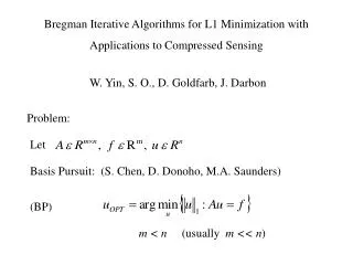
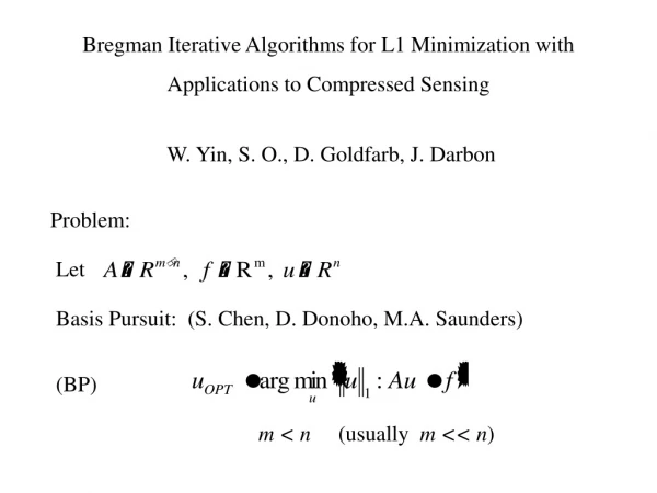
Bregman Iterative Algorithms for L1 Minimization with Applications to Compressed Sensing W. Yin, S. O., D. Goldfarb, J. Darbon Problem: Let Basis Pursuit: (S. Chen, D. Donoho, M.A. Saunders) (BP) m < n (usually m << n)
Basis Pursuit Arises in Compressed Sensing: (Candes, Romberg, Tao, Donoho, Tanner, Tsaig, Rudelson, Vershynin, Tropp) Fundamental principle: Through optimization, the sparsity of a signal can be exploited for signal recovery from incomplete measurements Let be highly sparse i.e.
Principle: Encode by Then recover from f by solving basis pursuit
Proven: [Candes, Tao] Recovery is perfect, whenever k,m,n satisfy certain conditions Type of matrices A allowing high compression rations (m << n) include • Random matrices with i.i.d. entries • Random ensembles of orthonormal transforms (e.g. matrices formed from random sets of the rows of Fourier transforms)
Huge number of potential applications of compressive sensing See e.g. Rich Baraniuk’s website: www.dsp.ece.rice.edu/cs/ minimization is widely used for compressive imaging, MRI and CT, multisensor networks and distributive sensing, analog-to-information conversion and biosensing (BP) can be transformed into a linear program, then solved by conventional methods. Not tailored for A large scale; dense; Also doesn’t use orthonormality for a Fourier matrix, etc.
One might solve the unconstrained problem (UNC) Need to be small to heavily weight the fidelity term. Also the solution to (UNC) never is that of (BP) unless f = 0 Here: Using Bregman iteration regularization we solve (BP) by a very small number of solutions to (UNC) with different values of f.
Method involves only • Matrix-vector multiplications • Component-wise shrinkages Method generalizes to the constrained problem For other convex J Can solve this through a finite number of Bregman iterations of (again, with a sequence of “f ” values)
Also: we have a two-line algorithm only involving matrix-vector multiplication and shrinkage operators generating {uk} that converges rapidly to an approximate solution of (BP) In fact the numerical evidence is overwhelming that it converges to a true solution if is large enough. Also: Algorithms are robust with respect to noise, both experimentally and with theoretical justification.
Background To solve (UNC): Figueiredo, Nowak and Wright Kim, Koh, Lustig and Boyd van den Berg and Friedlander Shrinkage (soft thresholding) with iteration used by: Chambolle, DeVore, Lee and Lucier Figueiredo and Nowak Daubechies, De Frise and DeMul Elad, Matalon and Zibulevsky Hale, Yin and Zhang Darbon and Osher Combettes and Pesquet
The shrinkage people developed an algorithm to solve for convex differentiable H(•) and get an iterative scheme: Since u is component-wise separable, we can solve by scalar shrinkage. Crucial for the speed!
where for y, R, define i.e., make this a semi-implicit method (in numerical analysis terms) Or replace H(u) by first order Taylor expansion at uk: and force u to be close to ukby the penalty term
This was adapted for solving and the resulting “linearized” approach was solved by a graph|network based algorithm, very fast. Darbon and Osher; Wang, Yin and Zhang. Also: Darbon and Osher did the linearized Bregman approached described here, but for TV deconvolution:
Bregman Iterative Regularization (Bregman 1967) Introduced by Osher, Burger, Goldfarb, Xu and Yin in an image processing context. Extended the Rudin-Osher-Fatemi model (ROF): b a noisy measurement of a clean image and is a tuning parameter. They used the Bregman distance based on
Not a distance really (unless J is quadratic) However for all w on the line segment connecting u and v. Instead of solving (ROF) once, our Bregman iterative regularization procedure solves (BROF) for starting with u0 = 0, p0 = 0 (gives (ROF) for u1) The p is automatically chosen from optimality
Difference is in the use of regularization. Bregman iterative regularization regularizes by minimizing the total variation based Bregman distance from u to the previous uk Earlier results: • converges monotonically to zero • ukgets closer to the unknown noisy image in the sense of Bregman distance diminishes in k at least as long as Numerically, it’s a big improvement.
For all k (BROF), the iterative procedure, can be reduced to ROF with the input i.e. add back the noise. This is totally general. Algorithm: Bregman iterative regularization (for J(u), H(u) convex, H differentiable) Results: The iterative sequence {uk} solves: (1) Monotonic decrease in H: (2) Convergence to the original in H with exact data:
(3) Approach towards the original in D with noisy data Let and suppose represent noisy data, noiseless data, perfect recovery, and noise level); then as long as
Motivation: Xu, Osher (2006) Wavelet based denoising with {j} a wavelet basis. Then solve Decouples: (observed (1998) by Chambolle, DeVore, Lee and Lucier)
This is soft thresholding Interesting: Bregman iterations give i.e. firm thresholding So for Bregman iterations it takes iterations to recover Spikes return in decreasing orders of their magnitudes and sparse data comes back very quickly.
Next: Simple case where Obvious solution: ajis component of a with largest magnitude.
assume aj = a1 > 0, f > 0 and a1strictly greater than all the other a. Then It is easy to see that the Bregman iterations give an exact solution in steps! This helps explain our success in the general case.
Convergence results: Again, the procedure Here Recent fast method (FPC) of Hale, Yin, Zhang to compute
This is nonlinear Bregman. Converges in a few iterations. However, even faster is linearized Bregman (Darbon-Osher, use for TV deblurring) described below 2 LINE CODE For nonlinear Bregman Theorem: Suppose an iterate uk satisfies Auk = f. Then uk solves (BP). Proof: By nonegativity of the Bregman distance, for any u
Theorem There exists an integer K < such that any is a solution of (BP) Idea: uses the fact that Works if we replace by for all k.
For dense Gaussian matrices A, we can solve large scale problem instances with more than 8 106 nonzeros in A e.g. n m 4096 2045 in 11 seconds. For partial DCT matrices, much faster 1,000,000 600,000 in 7 minutes But more like 40 seconds for the linearized Bregman approach! Also, can’t use minimizer for very small. Takes too long Need Bregman
Extensions Finite Convergence Let be convex on H, Hilbert space,
Thm: Let H(u) = h(Au – f), h convex, differentiable nonnegative, vanishing only at 0. Then Bregman iteration returns a solution of under very general conditions. Idea: then etc.
Strictly convex cases e.g. regularize, for Then Let Simple to prove.
Theorem: the decays exponentially to zero and easy.
Linearized Bregman Started with Osher-Darbon let Differs from standard Bregman because we replace by the sum of its first order approximation at uk and on proximity term at uk. Then we can use fast methods, either graph cuts for TV or shrinkage for to solve the above!!
yields Consider (BP). Let
Get a 2 line code: Linearized Bregman: Two Lines Matrix multiplication and scalar shrinkage.
Theorem: Let J be strictly convex and C2 and uOPT an optimal solution of Then if uk w we have decays exponentially if Proof is easy So for J(u) = |u|1this would mean that w approaches a minimize of ||u||1 subject to Au = f, as .
Theorem: (don’t need strict convexity and smoothness of J for this) then Proof easily follows from Osher, Burger, Goldfarb, Xu, Yin.
(again, don’t need strict convexity and smoothness) NOISE: Theorem (follows Bachmyer) Then the generalized Bregman distance diminishes with increasing k, as long as:
i.e. as long as the error Auk – f is not too small compared to the error in the “denoised” solution Of course if is the solution of the Basis Pursuit problem, then this Bregman distance monotonically decreases.
Note, this means for Basis Pursuit is diminishing for these values of k. Here belongs to [-1,1], determined by the iterative procedure.