Compressed Sensing MRI 2016.12.15
970 likes | 1.41k Vues
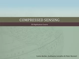
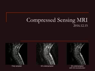
Compressed Sensing MRI 2016.12.15. Fully sampled. 6X undersampled. 6X undersampled with CS reconstruction. Lossy compression 失真壓縮. Reducing data size at cost of fidelity Widespread applied to music, images and movies: MP3, JPEG, H.264 (mpeg)

Compressed Sensing MRI 2016.12.15
E N D
Presentation Transcript
Compressed Sensing MRI2016.12.15 Fully sampled 6X undersampled 6X undersampledwith CS reconstruction
Lossy compression 失真壓縮 • Reducing data size at cost of fidelity • Widespread applied to music, images and movies: MP3, JPEG, H.264 (mpeg) • Most useful data are highly compressible (link) • Current model of data flow Acquisition Compression Application First lady of the Internet Lose 96% weight All bits of data are equal, but some bits are more equal than others.
勝 Lossy compression 失真壓縮 At cost of fidelity??? 14.8 kB Low resolution No compression Lossy compression “High” fidelity High resolution with “less” fidelity 2.2 kB 2.2 kB
-128 +127 Compressibility and Sparsity Sparse: most numbers are zero or close to zero 0 x 0.81 = x -0.45 = x -0.09 = x -0.04 = x -0.02 = x 0.007 = x 0.0006 = x 0 = x 0 = = -0.56 x = 0.31 x = 0.087 x = -0.003 x = 0.0001 x = 0 x = -0.38 x = 0.12 x = 0.0002 x = 0 x For example, under 2D “discrete cosine transform” (JPEG 1992)
Compressibility and Sparsity -128 +127 Sparse: most numbers are zero or close to zero 0 x 0.81 = x -0.45 = x -0.09 = x -0.04 = x -0.02 = x 0.007 = x 0.0006 = x 0 = x 0 = = -0.56 x = 0.31 x = 0.087 x = -0.003 x = 0.0001 x = 0 x = -0.38 x = 0.12 x = 0.0002 x = 0 x Compression by discard small component of discrete cosine transform.
MR medical images are sparse Sparse after wavelet transform Sparse after finite difference transform Sparse after Fourier transform in time
-128 +127 Noncompressible image 0 x 0.62 = x -0.60 = x -0.59 = x -0.56 = x -0.56 = x 0.54 = x 0.52 = x 0.52 = x 0.52= = -0.48 x = 0.46 x = 0.40 x = -0.35 x = 0.32 x = 0.32 x = -0.38 x = 0.32 x = 0.30 x = 0.24 x White noise is not sparse to any transform, include DCT.
Compressed sensing (CS) • Current model of data flow • Compressed sensing data flow Compressed sensing Acquisition Compression Application Application First lady of the Internet Lose 96% weight Already compressed
Compressed sensing (CS) • Current model gathers much more data than needed. Most could be discarded safely • Acquisition device must be fast, cheap, plenty • MR machine is slow, costly, scarce • Exploit image sparsity, CS MRI is possible Compressed sensing Application Already compressed
A crash course of MRI principle k space image Data acquisition DFT
A crash course of MRI principle k space Data acquisition
A crash course of MRI principle k space Data acquisition
A crash course of MRI principle k space Data acquisition
A crash course of MRI principle k space Data acquisition
A crash course of MRI principle k space Data acquisition
A crash course of MRI principle k space Data acquisition
A crash course of MRI principle k space Data acquisition
A crash course of MRI principle k space image Data acquisition DFT
Reconstruction with partial information Recovery? DFT missing data
Reconstruction with partial information Recovery? DFT a priori knowledge
Reconstruction with partial information Recovery? DFT DWT The a priori knowledge of compressed sensing is assumingthedata is sparsein some basis, such as wavelet basis. sparse
It seems very difficult…. • Alice • Bob • Eve The a priori knowledge of compressed sensing is assumingthedata is sparsein some basis, such as wavelet basis.
Localization make thing easier…. • 小王 (大喬 飾) • 小柯 (小喬 飾) • 小黃(由各位飾演) The a priori knowledge of compressed sensing is assumingthedata is sparsein some basis, such as wavelet basis.
Compressed sensing: minimal example 「這年頭,想要在海外置產不容易。如果小柯你海外豪宅分我一半,我就有十一棟了。」 『小王,不要太貪心。我們兩人的海外豪宅,總共比我的助理多十二棟呢。』 「噓,小黃正在偷聽,別再說了。再見。」
Compressed sensing: minimal example 「這年頭,想要在海外置產不容易。如果小柯你海外豪宅分我一半,我就有十一棟了。」 『小王,不要太貪心。我們兩人的海外豪宅,總共比我的助理多十二棟呢。』 「噓,小黃正在偷聽,別再說了。再見。」 • 小王 + ½小柯 = 11 • 小王 + 小柯 - 助理 = 12 • How many does each have? • 2 equations with 3 unknowns, many solutions exist
Compressed sensing: minimal example 「這年頭,想要在海外置產不容易。如果小柯你海外豪宅分我一半,我就有十一棟了。」 『小王,不要太貪心。我們兩人的海外豪宅,總共比我的助理多十二棟呢。』 「噓,小黃正在偷聽,別再說了。再見。」 • 小王 + ½小柯 = 11 • 小王 + 小柯 - 助理 = 12 • Oversea mansions are sparse • Sparse: most numbers are zero or close to zero • The sparsest solution:
ℓ0 , ℓ1 and ℓ2 (pseudo)norms This solution is minimal in ℓ0 and ℓ1 (pseudo)norm, but not in ℓ2 norm. • ℓ0pseudonorm: number of nonzero components • This is the definition of sparsity • ℓ1norm: sum of all components • The sparsest solution is minimal in ℓ1“incidentally” • ℓ2 norm: root of sum-squares
Incoherence • What if the scenario is: • 「小柯,我知道你的海外豪宅有兩棟。」 • 『但是我的助理一棟都沒有。』 • We will never know how much does 小王 has • Incoherence: Each sampled data should involves the basis as evenly as possible in the transformed domain • Random sampling is incoherent relative to any basis, but not always applicable
如果各位要寫作業的話… • Sparsity: few nonzero components in the transformed domain • Incoherence: Each sampled data should involves the basis as evenly as possible in the transformed domain • Incoherence and sparsity are the keys to successful compressed sensing
How much sampling is enough? • Signal size: n • Sampling number: m Nyquist sampling For example, n = 512 x 512 = 262,144, log n = 5.4
How much sampling is enough? • Signal size: n • Sampling number: m • Sparse: S nonzero component Nyquist sampling “Just enough” sampling For example, n = 512 x 512 = 262,144, log n = 5.4
How much sampling is enough? • Signal size: n • Sampling number: m • Sparse: S nonzero component • Incoherence: u • u = 1 maximally incoherent, usually u ~ 2 Nyquist sampling Compressed sensing “Just enough” sampling For example, n = 512 x 512 = 262,144, log n = 5.4
Compressed sensing, theorem 1 • Randomly acquiring m samples, m > a (strictly) S-sparse signal is recovered with probability > 1- Find k inRn Minimize || DWT(DFT(k)) ||1 Subject to ki = Ki i = 1… m Convex optimization problem Efficient algorithm exists
Compressed sensing, theorem 1 DFT DWT sparse Find k inRn Minimize || DWT(DFT(k)) ||1 Subject to ki = Ki i = 1… m Convex optimization problem Efficient algorithm exists
Compressed sensing, theorem 1 • Randomly acquiring m samples, m > a (strictly) S-sparse signal is recovered with probability > 1- What if the signal is only approximately S-sparse, and noisy?
Compressed sensing, theorem 2 approx. S-sparse recovery error noisy level Find k inRn Minimize || DWT(DFT(k)) ||1 Subject to ki≒Ki i = 1… m Convex optimization problem Efficient algorithm
Point spread function (PSF) in 1-dimension: Thresholding Thresholding random sampling Ambiguity! Regular sampling Imaging space k-space 模擬 subsampling所產生的雜訊 “模擬 subsampling 所產生的雜訊”: Point spread function The more evenly spread out of the noise, the better.
Point spread functionin 2-dimension “模擬 subsampling 所產生的雜訊”: Point spread function The more evenly spread out of the noise, the better: incoherence
Incoherent sampling: PSF in 2-dimension “模擬 subsampling 所產生的雜訊”: Point spread function The more evenly spread out of the noise, the better: incoherence
Summary of compressed sensing MRI • MRI images are sparse • Nonrandom incoherent k-space trajectories • Compressed sensing can achieve similar images quality using sub-Nyquist sampling • 5X to 10X speed up • Advantages…
Summary of compressed sensing MRI • MRI images are sparse • Nonrandom incoherent k-space trajectories • Compressed sensing can achieve similar images quality using sub-Nyquist sampling • 5X to 10X speed up Make time-consuming scan probable More NEX One breath-hold body images Ultrafast screening for stroke No motion artifact No anesthesia for babies No more overtime work Larger FOV Higher resolution
What’s next? Beyond sparsity • Sparsity is a rudimentary a priori knowledge • Can we expand a priori knowledge by machine learning? • Beyond sparsity
It’s Showtime! Original image 6X subsampling with CS Original 6X subsampling
It’s Showtime! Original image 6X subsampling with CS Original 6X subsampling
It’s Showtime! Free breathingwhole liver perfusion One breath-holdwhole heart perfusion