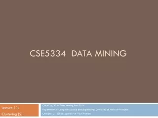
CSE5334 Data Mining
CSE5334 Data Mining. Lecture 3: Data Warehousing, OLAP, Data Cube. CSE 4392/5334 Data Mining, Fall 2014 Department of Computer Science and Engineering, University of Texas at Arlington Chengkai Li (Slides courtesy of Jiawei Han).

CSE5334 Data Mining
E N D
Presentation Transcript
CSE5334 Data Mining Lecture 3: Data Warehousing, OLAP, Data Cube CSE 4392/5334 Data Mining, Fall 2014 Department of Computer Science and Engineering, University of Texas at Arlington Chengkai Li (Slides courtesy of Jiawei Han)
Chapter 3: Data Warehousing and OLAP Technology: An Overview • What is a data warehouse? • A multi-dimensional data model • Data warehouse architecture • Data warehouse implementation
What is Data Warehouse? • “A data warehouse is asubject-oriented, integrated, time-variant, and nonvolatilecollection of data in support of management’s decision-making process.”—W. H. Inmon • Data warehousing: The process of constructing and using data warehouses
Data Warehouse—Subject-Oriented • Organized around major subjects, such as customer, product, sales • Focusing on the modeling and analysis of data for decision makers, not on daily operations or transaction processing • Provide a simple and concise view around particular subject issues by excluding data that are not useful in the decision support process
Data Warehouse—Integrated • Constructed by integrating multiple, heterogeneous data sources • relational databases, flat files, on-line transaction records • Data cleaning and data integration techniques are applied. • Ensure consistency in naming conventions, encoding structures, attribute measures, etc. among different data sources • E.g., Hotel price: currency, tax, breakfast covered, etc. • When data is moved to the warehouse, it is converted.
Data Warehouse—Time Variant • The time horizon for the data warehouse is significantly longer than that of operational systems • Operational database: current value data • Data warehouse data: provide information from a historical perspective (e.g., past 5-10 years) • Every key structure in the data warehouse • Contains an element of time, explicitly or implicitly • But the key of operational data may or may not contain “time element”
Data Warehouse—Nonvolatile • A physically separate store of data transformed from the operational environment • Operational update of data does not occur in the data warehouse environment • Does not require transaction processing, recovery, and concurrency control mechanisms • Requires only two operations in data accessing: • initial loading of data and access of data
Data Warehouse vs. Operational DBMS • OLTP (on-line transaction processing) • Major task of traditional relational DBMS • Day-to-day operations: purchasing, inventory, banking, manufacturing, payroll, registration, accounting, etc. • OLAP (on-line analytical processing) • Major task of data warehouse system • Data analysis and decision making • Distinct features (OLTP vs. OLAP): • User and system orientation: customer vs. market • Data contents: current, detailed vs. historical, consolidated • Database design: ER + application vs. star + subject • View: current, local vs. evolutionary, integrated • Access patterns: update vs. read-only but complex queries
Why Separate Data Warehouse? • Different functions and different data: • Note: There are more and more systems which perform OLAP analysis directly on relational databases • There is no absolute boundary.
Chapter 3: Data Warehousing and OLAP Technology: An Overview • What is a data warehouse? • A multi-dimensional data model • Data warehouse architecture • Data warehouse implementation
Data Cube • A data warehouse is based on a multidimensional data model which views data in the form of a data cube • A data cube contains aggregates of measure values, on various combinations of dimensions, and furthermore, with various levels of aggregation on individual dimension. • In data warehousing literature, an n-D base cube is called a base cuboid. The top most 0-D cuboid, which holds the highest-level of summarization, is called the apex cuboid. The lattice of cuboids forms a data cube.
A 3-D Cuboid • Sales volume as a function of product, month, and region Dimensions: Product, Location, Time Hierarchical summarization paths Location (Region) Industry Region Year Category Country Quarter Item City Month Week Office Day Product (Item) Time (Month)
Time (Quarter) 2Qtr 1Qtr sum 3Qtr 4Qtr Product (category) TV U.S.A PC VCR sum Location (country) Canada Mexico sum All, All, All An Example of Data Cube Total annual sales of TV in U.S.A.
Data Cube: A Lattice of Cuboids all 0-D(apex) cuboid location product time 1-D cuboids product,time product,location time, location 2-D cuboids 3-D(base) cuboid product, time, location
Time (Quarter) 2Qtr 1Qtr sum 3Qtr 4Qtr Product (category) TV PC U.S.A VCR sum Location (country) Canada Mexico sum All, All, All Cuboids all location product time time, location product,location Total annual sales of TV in U.S.A. product,time product, time, location
all 0-D(apex) cuboid time product location supplier 1-D cuboids time,location product, location location,supplier 2-D cuboids time,supplier product,supplier time,location,supplier 3-D cuboids product,location,supplier time,product,supplier 4-D(base) cuboid Another 4-D Data Cube time,product time,product,location time, product, location, supplier
A Concept Hierarchy on Location Dimension all all Europe ... North_America region Germany ... Spain Canada ... Mexico country Vancouver ... city Frankfurt ... Toronto L. Chan ... M. Wind office
Concept Hierarchy in Data Cube all Product (category) Time (quarter) Location (country) Product(category), location (country) Location (city) Product(category), Time(quarter) Time(quarter), Location(country) Product(category), location (city) Product(category), Time(quarter), Location(country) Time(quarter), Location(city) Product(category), Time(quarter), Location(city)
Conceptual Schema Design • Dimensions & Measures • Dimension tables, such as product (item_name, brand, type), or time(day, week, month, quarter, year) • Fact table contains measures (such as dollars_sold) and keys to each of the related dimension tables
Conceptual Modeling of Data Warehouses • Star schema: A fact table in the middle connected to a set of dimension tables
item time item_key item_name brand type supplier_type time_key day day_of_the_week month quarter year location branch location_key street city state_or_province country branch_key branch_name branch_type Example of Star Schema Sales Fact Table time_key item_key branch_key location_key units_sold dollars_sold avg_sales Measures
Conceptual Modeling of Data Warehouses • Snowflake schema: A refinement of star schema where some dimensional hierarchy is normalized into a set of smaller dimension tables, forming a shape similar to snowflake It provides explicit support of hierarchy • Easier to manage the dimension • Can be less efficient (due to join) than star schema
supplier item time item_key item_name brand type supplier_key supplier_key supplier_type time_key day day_of_the_week month quarter year city location branch city_key city state_or_province country location_key street city_key branch_key branch_name branch_type Example of Snowflake Schema Sales Fact Table time_key item_key branch_key location_key units_sold dollars_sold avg_sales Measures
Conceptual Modeling of Data Warehouses • Fact constellations: Multiple fact tables share dimension tables, viewed as a collection of stars, therefore called galaxy schema or fact constellation
item time item_key item_name brand type supplier_type time_key day day_of_the_week month quarter year location location_key street city province_or_state country shipper branch shipper_key shipper_name location_key shipper_type branch_key branch_name branch_type Example of Fact Constellation Shipping Fact Table time_key Sales Fact Table item_key time_key shipper_key item_key from_location branch_key to_location location_key dollars_cost units_sold units_shipped dollars_sold avg_sales Measures
Measures of Data Cube: Three Categories • Distributive: if the result derived by applying the function to n aggregate values is the same as that derived by applying the function on all the data without partitioning • E.g., count(), sum(), min(), max() • Algebraic:if it can be computed by an algebraic function with M arguments (where M is a bounded integer), each of which is obtained by applying a distributive aggregate function • E.g.,avg(), min_N(), standard_deviation() • Holistic: if there is no constant bound on the storage size needed to describe a subaggregate. • E.g., median(), mode(), rank()
Typical OLAP Operations • Roll up (drill-up): summarize data • by climbing up hierarchy or by dimension reduction • Drill down (roll down): reverse of roll-up • from higher level summary to lower level summary or detailed data, or introducing new dimensions • Slice and dice:project and select • Pivot (rotate): • reorient the cube, visualization, 3D to series of 2D planes
Roll up and Drill Down • Roll up: increasing the level of aggregation • further aggregating along one more dimension • or further aggregating along the hierarchy of one dimension • Drill down: decreasing the level of aggregating It is like traversing in the lattice of cuboids.
Chapter 3: Data Warehousing and OLAP Technology: An Overview • What is a data warehouse? • A multi-dimensional data model • Data warehouse architecture • Data warehouse implementation
OLAP Server Architectures • Relational OLAP (ROLAP) • Use relational or extended-relational DBMS to store and manage warehouse data and OLAP middle ware • Include optimization of DBMS backend, implementation of aggregation navigation logic, and additional tools and services • Greater scalability • Multidimensional OLAP (MOLAP) • Sparse array-based multidimensional storage engine • Fast indexing to pre-computed summarized data • Hybrid OLAP (HOLAP)(e.g., Microsoft SQLServer) • Flexibility, e.g., low level: relational, high-level: array • Specialized SQL servers (e.g., Redbricks) • Specialized support for SQL queries over star/snowflake schemas
Chapter 3: Data Warehousing and OLAP Technology: An Overview • What is a data warehouse? • A multi-dimensional data model • Data warehouse architecture • Data warehouse implementation
Efficient Data Cube Computation • Data cube can be viewed as a lattice of cuboids • The bottom-most cuboid is the base cuboid • The top-most cuboid (apex) contains only one cell • How many cuboids in an n-dimensional cube with L levels? • Materialization of data cube • Materialize every (cuboid) (full materialization), none (no materialization), or some (partial materialization) • Selection of which cuboids to materialize • Based on size, sharing, access frequency, etc.
Indexing OLAP Data: Bitmap Index • Index on a particular column • Each value in the column has a bit vector: bit-op is fast • The length of the bit vector: # of records in the base table • The i-th bit is set if the i-th row of the base table has the value for the indexed column • not suitable for high cardinality domains Base table Index on Region Index on Type
Indexing OLAP Data: Join Indices • Join index: JI(R-id, S-id) where R (R-id, …) S (S-id, …) • Traditional indices map the values to a list of record ids • It materializes relational join in JI file and speeds up relational join • In data warehouses, join index relates the values of the dimensions of a start schema to rows in the fact table. • E.g. fact table: Sales and two dimensions city and product • A join index on city maintains for each distinct city a list of R-IDs of the tuples recording the Sales in the city • Join indices can span multiple dimensions
Efficient Processing OLAP Queries • Determine which operations should be performed on the available cuboids • Transform drill, roll, etc. into corresponding SQL and/or OLAP operations, e.g., dice = selection + projection • Determine which materialized cuboid(s) should be selected for OLAP op. • Let the query to be processed be on {brand, province_or_state} with the condition “year = 2004”, and there are 4 materialized cuboids available: 1) {year, item_name, city} 2) {year, brand, country} 3) {year, brand, province_or_state} 4) {item_name, province_or_state} where year = 2004 Which should be selected to process the query? • Explore indexing structures and compressed vs. dense array structures in MOLAP
Chapter 3: Data Warehousing and OLAP Technology: An Overview • What is a data warehouse? • A multi-dimensional data model • Data warehouse architecture • Data warehouse implementation • Summary
Summary: Data Warehouse and OLAP Technology • Why data warehousing? • A multi-dimensional model of a data warehouse • Star schema, snowflake schema, fact constellations • A data cube consists of dimensions & measures • OLAP operations: drilling, rolling, slicing, dicing and pivoting • Data warehouse architecture OLAP servers: ROLAP, MOLAP, HOLAP • Efficient computation of data cubes • Partial vs. full vs. no materialization • Indexing OALP data: Bitmap index and join index • OLAP query processing