
MGMG 522 : Session #7 Serial Correlation
E N D
Presentation Transcript
Serial Correlation (a.k.a. Autocorrelation) • Autocorrelation is a violation of the classical assumption #4 (error terms are uncorrelated with each other). • Autocorrelation can be categorized into 2 kinds: • Pure autocorrelation (autocorrelation that exists in a correctly specified regression model). • Impure autocorrelation (autocorrelation that is caused by specification errors: omitted variables or incorrect functional form). • Autocorrelation mostly happens in a data set where order of observations has some meaning (e.g. time-series data).
Pure Autocorrelation • Classical assumption #4 implies that there is no correlation between any two observations of the error term, or E(rij) = 0 for i ≠ j. • Most common kind of autocorrelation is the first-order autocorrelation, where current observation of the error term is correlated with the previous observation of the error term. • Mathematically, εt = εt-1 + ut. Where, ε = error term, = simple correlation coefficient (-1 < < +1), and u = classical error term.
(pronounced “rho”) • -1 < < +1 • < 0 indicates negative autocorrelation (the signs of the error term switch back and forth). • > 0 indicates positive autocorrelation (a positive error term tends to be followed by a positive error term and a negative error term tends to be followed by a negative error term). • Positive autocorrelation is more common than negative autocorrelation.
Higher-order Autocorrelation • Examples: • Seasonal autocorrelation: εt = εt-4 + ut • Second-order autocorrelation: εt = 1εt-1 + 2εt-2 + ut.
Impure Autocorrelation • Caused by specification errors: omitted variables or incorrect functional form. • Specification errors should be corrected first by way of investigating the independent variables and/or functional form. • How can omitted variables or incorrect functional form cause autocorrelation? • Remember that the error term is the sum of the effects of: • Omitted variables • Nonlinearities • Measurement errors • Pure error
Example: Omitted VariableCauses Autocorrelation • Correct model: Y = 0+1X1+2X2+ε • If X2 is omitted: Y = 0+1X1+ε* • Where, ε* = 2X2+ε • If ε is small compared to 2X2, and X2 is serially correlated (very likely in a time series), ε* will be autocorrelated. • Estimate of 1will be biased (because X2 is omitted). • Both the bias and impure autocorrelation will disappear once the model gets corrected.
Example: Incorrect Functional Form Causes Autocorrelation • Correct model: Y = 0+1X1+2X12+ε • Our model: Y = 0+1X1+ε* • Where, ε* = 2X12+ε • Autocorrelation could result. (See Figure 9.5 on p. 323)
Consequences of Autocorrelation • Pure autocorrelation does not cause bias in the coefficient estimates. • Pure autocorrelation increases variances of the coefficient estimates. • Pure autocorrelation causes OLS to underestimate the standard errors of the coefficients. (Hence, pure autocorrelation overestimates the t-values.)
Example of the Consequences • With no autocorrelation • b1 = 0.008 • SE(b1) = 0.002 • t-value = 4.00 • With autocorrelation but a correct SE of coefficient • b1 = 0.008 • SE*(b1) = 0.006 • t-value = 1.33 • With autocorrelation and OLS underestimate SE of coefficient • b1 = 0.008 • SE(b1) = 0.003 • t-value = 2.66
Detection of Autocorrelation • Use the Durbin-Watson d Test • Durbin-Watson d Test is only appropriate for • a regression model with an intercept term, • autocorrelation is of first-order, and • The regression model does not include a lagged dependent variable as an independent variable (e.g., Yt-1) • Durbin-Watson d statistic for T observations is:
d statistic • d = 0 indicates extreme positive autocorrelation (et = et-1). • d = 4 indicates extreme negative autocorrelation (et = -et-1). • d = 2 indicates no autocorrelation Σ(et-et-1)2 = Σ(et2-2etet-1+et-12) = Σ(et2+et-12).
The Use of d Test • Econometricians almost never test one-sided that there is negative autocorrelation. Most of the tests are to detect positive autocorrelation (one-sided) or to detect autocorrelation (two-sided). • d test is sometimes inconclusive.
Example: One-sided d test that there is positive autocorrelation H0: ≤ 0 (no positive autocorrelation) H1: > 0 (positive autocorrelation) • Decision Rule If d < dL Reject H0 If d > dU Do not reject H0 If dL ≤ d ≤ dU Inconclusive
Example: Two-sided d test that there is autocorrelation H0: = 0 (no autocorrelation) H1: ≠ 0 (autocorrelation) • Decision Rule If d < dL Reject H0 If d > 4-dL Reject H0 If 4-dU > d > dU Do not reject H0 Otherwise Inconclusive
Correcting Autocorrelation • Use the Generalized Least Squares to restore the minimum variance property of the OLS estimation.
GLS properties • Now, the error term is not autocorrelated. Thus, OLS estimation of Eq.4 will be minimum variance. • The slope coefficient 1 of Eq.1 will be the same as that of Eq.4, and has the same meaning. • Adj-R2 from Eq.1 and Eq.4 should not be used for comparison because the dependent variables are not the same in the two models.
GLS methods • Use the Cochrane-Orcutt method (EViews does not support this estimation method.) (Details on p. 331-333) • Use the AR(1) method (In EViews, insert the term AR(1) after the list of independent variables.) • When d test is inconclusive, GLS should not be used. • When d test is conclusive, GLS should not be used if • The autocorrelation is impure. • The consequence of autocorrelation is minor.
Autocorrelation-Corrected Standard Errors • The idea of this remedy goes like this. • Since, there is no bias in the coefficient estimates. • But, the standard errors of the coefficient estimates are larger with autocorrelation than without it. • Therefore, why not fix the standard errors and leave the coefficient estimates alone? • This method is referred to as HCCM (heteroskedasticity-consistent covariance matrix).
Autocorrelation-Corrected Standard Errors • In EViews, you will choose “LS” and click on “Options”, then select “Heteroskedasticity-Consistent Coefficient Covariance” and select “Newey-West”. • The standard errors of the coefficient estimates will be bigger than those from the OLS. • Newey-West standard errors are also known as HAC standard errors; for they correct both Heteroskedasticity and AutoCorrelation problems. • This method works best in a large sample data. In fact, when the sample size is large, you can always use HAC standard errors.