N-Gram Language Models
N-Gram Language Models. CMSC 723: Computational Linguistics I ― Session #9. Jimmy Lin The iSchool University of Maryland Wednesday, October 28, 2009. N-Gram Language Models. What? LMs assign probabilities to sequences of tokens Why? Statistical machine translation Speech recognition

N-Gram Language Models
E N D
Presentation Transcript
N-Gram Language Models CMSC 723: Computational Linguistics I ― Session #9 Jimmy Lin The iSchool University of Maryland Wednesday, October 28, 2009
N-Gram Language Models • What? • LMs assign probabilities to sequences of tokens • Why? • Statistical machine translation • Speech recognition • Handwriting recognition • Predictive text input • How? • Based on previous word histories • n-gram = consecutive sequences of tokens
Huh? Noam Chomsky Fred Jelinek But it must be recognized that the notion “probability of a sentence” is an entirely useless one, under any known interpretation of this term. (1969, p. 57) Anytime a linguist leaves the group the recognition rate goes up. (1988) Every time I fire a linguist…
N-Gram Language Models N=1 (unigrams) This is a sentence Unigrams: This, is, a, sentence Sentence of length s, how many unigrams?
N-Gram Language Models N=2 (bigrams) This is a sentence Bigrams: This is, is a, a sentence Sentence of length s, how many bigrams?
N-Gram Language Models N=3 (trigrams) This is a sentence Trigrams: This is a, is a sentence Sentence of length s, how many trigrams?
[chain rule] Computing Probabilities Is this practical? No! Can’t keep track of all possible histories of all words!
Approximating Probabilities Basic idea: limit history to fixed number of words N (Markov Assumption) N=1: Unigram Language Model Relation to HMMs?
Approximating Probabilities Basic idea: limit history to fixed number of words N (Markov Assumption) N=2: Bigram Language Model Relation to HMMs?
Approximating Probabilities Basic idea: limit history to fixed number of words N (Markov Assumption) N=3: Trigram Language Model Relation to HMMs?
Building N-Gram Language Models • Use existing sentences to compute n-gram probability estimates (training) • Terminology: • N = total number of words in training data (tokens) • V = vocabulary size or number of unique words (types) • C(w1,...,wk) = frequency of n-gram w1, ..., wk in training data • P(w1, ..., wk) = probability estimate for n-gram w1 ... wk • P(wk|w1, ..., wk-1) = conditional probability of producing wk given the history w1, ... wk-1 What’s the vocabulary size?
Vocabulary Size: Heaps’ Law • Heaps’ Law: linear in log-log space • Vocabulary size grows unbounded! Mis vocabulary size Tis collection size (number of documents) kand bare constants Typically, kis between 30 and 100, bis between 0.4 and 0.6
Heaps’ Law for RCV1 k = 44 b = 0.49 First 1,000,020 terms: Predicted = 38,323 Actual = 38,365 Reuters-RCV1 collection: 806,791 newswire documents (Aug 20, 1996-August 19, 1997) Manning, Raghavan, Schütze, Introduction to Information Retrieval (2008)
Building N-Gram Models • Start with what’s easiest! • Compute maximum likelihood estimates for individual n-gram probabilities • Unigram: • Bigram: • Uses relative frequencies as estimates • Maximizes the likelihood of the data given the model P(D|M) Why not just substitute P(wi) ?
<s> </s> <s> </s> <s> </s> Example: Bigram Language Model I am SamSam I am I do not like green eggs and ham Training Corpus P( I | <s> ) = 2/3 = 0.67 P( Sam | <s> ) = 1/3 = 0.33 P( am | I ) = 2/3 = 0.67 P( do | I ) = 1/3 = 0.33 P( </s> | Sam )= 1/2 = 0.50 P( Sam | am) = 1/2 = 0.50 ... Bigram Probability Estimates Note: We don’t ever cross sentence boundaries
Building N-Gram Models • Start with what’s easiest! • Compute maximum likelihood estimates for individual n-gram probabilities • Unigram: • Bigram: • Uses relative frequencies as estimates • Maximizes the likelihood of the data given the model P(D|M) Let’s revisit this issue… Why not just substitute P(wi) ?
More Context, More Work • Larger N = more context • Lexical co-occurrences • Local syntactic relations • More context is better? • Larger N = more complex model • For example, assume a vocabulary of 100,000 • How many parameters for unigram LM? Bigram? Trigram? • Larger N has another more serious and familiar problem!
Data Sparsity P( I | <s> ) = 2/3 = 0.67 P( Sam | <s> ) = 1/3 = 0.33 P( am | I ) = 2/3 = 0.67 P( do | I ) = 1/3 = 0.33 P( </s> | Sam )= 1/2 = 0.50 P( Sam | am) = 1/2 = 0.50 ... Bigram Probability Estimates P(I like ham) = P( I | <s> ) P( like | I ) P( ham | like ) P( </s> | ham ) = 0 Why? Why is this bad?
Data Sparsity • Serious problem in language modeling! • Becomes more severe as N increases • What’s the tradeoff? • Solution 1: Use larger training corpora • Can’t always work... Blame Zipf’s Law (Looong tail) • Solution 2: Assign non-zero probability to unseen n-grams • Known as smoothing
Smoothing • Zeros are bad for any statistical estimator • Need better estimators because MLEs give us a lot of zeros • A distribution without zeros is “smoother” • The Robin Hood Philosophy: Take from the rich (seen n-grams) and give to the poor (unseen n-grams) • And thus also called discounting • Critical: make sure you still have a valid probability distribution! • Language modeling: theory vs. practice
Laplace’s Law • Simplest and oldest smoothing technique • Just add 1 to all n-gram counts including the unseen ones • So, what do the revised estimates look like?
Laplace’s Law: Probabilities Unigrams Bigrams Careful, don’t confuse the N’s! What if we don’t know V?
Laplace’s Law: Frequencies Expected Frequency Estimates Relative Discount
Laplace’s Law • Bayesian estimator with uniform priors • Moves too much mass over to unseen n-grams • What if we added a fraction of 1 instead?
Lidstone’s Law of Succession • Add 0 < γ < 1 to each count instead • The smaller γ is, the lower the mass moved to the unseen n-grams (0=no smoothing) • The case of γ = 0.5 is known as Jeffery-Perks Law or Expected Likelihood Estimation • How to find the right value of γ?
Good-Turing Estimator • Intuition: Use n-grams seen once to estimate n-grams never seen and so on • Compute Nr (frequency of frequency r) • N0 is the number of items with count 0 • N1 is the number of items with count 1 • …
Good-Turing Estimator • For each r, compute an expected frequency estimate (smoothed count) • Replace MLE counts of seen bigrams with the expected frequency estimates and use those for probabilities
Good-Turing Estimator • What about an unseen bigram? • Do we know N0? Can we compute it for bigrams?
Good-Turing Estimator: Example N0 = (14585)2 - 199252 Cunseen = N1 / N0 = 0.00065 Punseen = N1/( N0N ) = 1.06 x 10⁻⁹ Note: Assumes mass is uniformly distributed V = 14585 Seen bigrams =199252 C(person she) = 2 CGT(person she) = (2+1)(10531/25413) = 1.243 C(person) = 223 P(she|person) =CGT(person she)/223 = 0.0056
Good-Turing Estimator • For each r, compute an expected frequency estimate (smoothed count) • Replace MLE counts of seen bigrams with the expected frequency estimates and use those for probabilities What if wi isn’t observed?
Good-Turing Estimator • Can’t replace all MLE counts • What about rmax? • Nr+1 = 0 for r = rmax • Solution 1: Only replace counts for r < k (~10) • Solution 2: Fit a curve S through the observed (r, Nr) values and use S(r) instead • For both solutions, remember to do what? • Bottom line: the Good-Turing estimator is not used by itself but in combination with other techniques
Combining Estimators • Better models come from: • Combining n-gram probability estimates from different models • Leveraging different sources of information for prediction • Three major combination techniques: • Simple Linear Interpolation of MLEs • Katz Backoff • Kneser-Ney Smoothing
Linear MLE Interpolation • Mix a trigram model with bigram and unigram models to offset sparsity • Mix = Weighted Linear Combination
Linear MLE Interpolation • λi are estimated on some held-out data set (not training, not test) • Estimation is usually done via an EM variant or other numerical algorithms (e.g. Powell)
Backoff Models • Consult different models in order depending on specificity (instead of all at the same time) • The most detailed model for current context first and, if that doesn’t work, back off to a lower model • Continue backing off until you reach a model that has some counts
Backoff Models • Important: need to incorporate discounting as an integral part of the algorithm… Why? • MLE estimates are well-formed… • But, if we back off to a lower order model without taking something from the higher order MLEs, we are adding extra mass! • Katz backoff • Starting point: GT estimator assumes uniform distribution over unseen events… can we do better? • Use lower order models!
Katz Backoff Given a trigram “x y z”
Katz Backoff (from textbook) Given a trigram “x y z” Typo?
Katz Backoff • Why use PGT and not PMLE directly ? • If we use PMLE then we are adding extra probability mass when backing off! • Another way: Can’t save any probability mass for lower order models without discounting • Why the α’s? • To ensure that total mass from all lower order models sums exactly to what we got from the discounting
Kneser-Ney Smoothing • Observation: • Average Good-Turing discount for r ≥ 3 is largely constant over r • So, why not simply subtract a fixed discount D (≤1) from non-zero counts? • Absolute Discounting: discounted bigram model, back off to MLE unigram model • Kneser-Ney: Interpolate discounted model with a special “continuation” unigram model
Kneser-Ney Smoothing • Intuition • Lower order model important only when higher order model is sparse • Should be optimized to perform in such situations • Example • C(Los Angeles) = C(Angeles) = M; M is very large • “Angeles” always and only occurs after “Los” • Unigram MLE for “Angeles” will be high and a normal backoff algorithm will likely pick it in any context • It shouldn’t, because “Angeles” occurs with only a single context in the entire training data
= number of different contexts wihas appeared in Kneser-Ney Smoothing • Kneser-Ney: Interpolate discounted model with a special “continuation” unigram model • Based on appearance of unigrams in different contexts • Excellent performance, state of the art • Why interpolation, not backoff?
Explicitly Modeling OOV • Fix vocabulary at some reasonable number of words • During training: • Consider any words that don’t occur in this list as unknown or out of vocabulary (OOV) words • Replace all OOVs with the special word <UNK> • Treat <UNK> as any other word and count and estimate probabilities • During testing: • Replace unknown words with <UNK> and use LM • Test set characterized by OOV rate (percentage of OOVs)
Evaluating Language Models • Information theoretic criteria used • Most common: Perplexity assigned by the trained LM to a test set • Perplexity: How surprised are you on average by what comes next ? • If the LM is good at knowing what comes next in a sentence ⇒ Low perplexity (lower is better) • Relation to weighted average branching factor
Computing Perplexity • Given testsetW with words w1, ...,wN • Treat entire test set as one word sequence • Perplexity is defined as the probability of the entire test set normalized by the number of words • Using the probability chain rule and (say) a bigram LM, we can write this as • A lot easer to do with log probs!
Training: N=38 million, V~20000, open vocabulary, Katz backoff where applicable Test: 1.5 million words, same genre as training Practical Evaluation • Use <s> and </s> both in probability computation • Count </s> but not <s> in N • Typical range of perplexities on English text is 50-1000 • Closed vocabulary testing yields much lower perplexities • Testing across genres yields higher perplexities • Can only compare perplexities if the LMs use the same vocabulary
Typical “State of the Art” LMs • Training • N = 10 billion words, V = 300k words • 4-gram model with Kneser-Ney smoothing • Testing • 25 million words, OOV rate 3.8% • Perplexity ~50
Take-Away Messages • LMs assign probabilities to sequences of tokens • N-gram language models: consider only limited histories • Data sparsity is an issue: smoothing to the rescue • Variations on a theme: different techniques for redistributing probability mass • Important: make sure you still have a valid probability distribution!