N-gram Models
N-gram Models. CMSC 25000 Artificial Intelligence March 1, 2005. Markov Assumptions. Exact computation requires too much data Approximate probability given all prior wds Assume finite history Bigram: Probability of word given 1 previous First-order Markov

N-gram Models
E N D
Presentation Transcript
N-gram Models CMSC 25000 Artificial Intelligence March 1, 2005
Markov Assumptions • Exact computation requires too much data • Approximate probability given all prior wds • Assume finite history • Bigram: Probability of word given 1 previous • First-order Markov • Trigram: Probability of word given 2 previous • N-gram approximation Bigram sequence
Evaluating n-gram models • Entropy & Perplexity • Information theoretic measures • Measures information in grammar or fit to data • Conceptually, lower bound on # bits to encode • Entropy: H(X): X is a random var, p: prob fn • Perplexity: • Weighted average of number of choices
Perplexity Model Comparison • Compare models with different history • Train models • 38 million words – Wall Street Journal • Compute perplexity on held-out test set • 1.5 million words (~20K unique, smoothed) • N-gram Order | Perplexity • Unigram | 962 • Bigram | 170 • Trigram | 109
Does the model improve? • Compute probability of data under model • Compute perplexity • Relative measure • Decrease toward optimum? • Lower than competing model?
Entropy of English • Shannon’s experiment • Subjects guess strings of letters, count guesses • Entropy of guess seq = Entropy of letter seq • 1.3 bits; Restricted text • Build stochastic model on text & compute • Brown computed trigram model on varied corpus • Compute (per-char) entropy of model • 1.75 bits
Using N-grams • Language Identification • Take text samples • English, French, Spanish, German • Build character tri-gram models • Test Sample: Compute maximum likelihood • Best match is chosen language • Authorship attribution
Sequence Models in Modern AI • Probabilistic sequence models: • HMMs, N-grams • Train from available data • Classification with contextual influence • Robust to noise/variability • E.g. Sentences vary in degrees of acceptability • Provides ranking of sequence quality • Exploits large scale data, storage, memory, CPU
Computer Vision CMSC 25000 Artificial Intelligence March 1, 2005
Roadmap • Motivation • Computer vision applications • Is a Picture worth a thousand words? • Low level features • Feature extraction: intensity, color • High level features • Top-down constraint: shape from stereo, motion,.. • Case Study: Vision as Modern AI • Fast, robust face detection (Viola & Jones 2002)
Perception • From observation to facts about world • Analogous to speech recognition • Stimulus (Percept) S, World W • S = g(W) • Recognition: Derive world from percept • W=g’(S) • Is this possible?
Key Perception Problem • Massive ambiguity • Optical illusions • Occlusion • Depth perception • “Objects are closer than they appear” • Is it full-sized or a miniature model?
Handling Uncertainty • Identify single perfect correct solution • Impossible! • Noise, ambiguity, complexity • Solution: • Probabilistic model • P(W|S) = αP(S|W) P(W) • Maximize image probability and model probability
Handling Complexity • Don’t solve the whole problem • Don’t recover every object/position/color… • Solve restricted problem • Find all the faces • Recognize a person • Align two images
Modern Computer Vision Applications • Face / Object detection • Medical image registration • Face recognition • Object tracking
Images and Representations • Initially pixel images • Image as NxM matrix of pixel values • Alternate image codings • Grey-scale intensity values • Color encoding: intensities of RGB values
Image Features • Grey-scale and color intensities • Directly access image signal values • Large number of measures • Possibly noisy • Only care about intensities as cues to world • Image Features: • Mid-level representation • Extract from raw intensities • Capture elements of interest for image understanding
Edge Detection • Find sharp demarcations in intensity • 1) Apply spatially oriented filters • E.g. vertical, horizontal, diagonal • 2) Label above-threshold pixels with edge orientation • 3) Combine edge segments with same orientation: line
Top-down Constraints • Goal: Extract objects from images • Approach: apply knowledge about how the world works to identify coherent objects; reconstruct 3D
Motion: Optical Flow • Find correspondences in sequential images • Units which move together represent objects
Edge-Based 2-3D Reconstruction Assume world of solid polyhedra with 3-edge vertices Apply Waltz line labeling – via Constration Satisfaction
Summary • Vision is hard: • Noise, ambiguity, complexity • Prior knowledge is essential to constrain problem • Cohesion of objects, optics, object features • Combine multiple cues • Motion, stereo, shading, texture, • Image/object matching: • Library: features, lines, edges, etc • Apply domain knowledge: Optics • Apply machine learning: NN, NN, CSP, etc
Computer Vision Case Study • “Rapid Object Detection using a Boosted Cascade of Simple Features”, Viola/Jones ’01 • Challenge: • Object detection: • Find all faces in an arbitrary images • Real-time execution • 15 frames per second • Need simple features, classifiers
Rapid Object Detection Overview • Fast detection with simple local features • Simple fast feature extraction • Small number of computations per pixel • Rectangular features • Feature selection with Adaboost • Sequential feature refinement • Cascade of classifiers • Increasingly complex classifiers • Repeatedly rule out non-object areas
Picking Features • What cues do we use for object detection? • Not direct pixel intensities • Features • Can encode task specific domain knowledge (bias) • Difficult to learn directly from data • Reduce training set size • Feature system can speed processing
Rectangle Features • Treat rectangles as units • Derive statistics • Two-rectangle features • Two similar rectangular regions • Vertically or horizontally adjacent • Sum pixels in each region • Compute difference between regions
Rectangle Features II • Three-rectangle features • 3 similar rectangles: horizontally/vertically • Sum outside rectangles • Subtract from center region • Four-rectangle features • Compute difference between diagonal pairs • HUGE feature set: ~180,000
Computing Features Efficiently • Fast detection requires fast feature calculation • Rapidly compute intermediate representation • “Integral image” • Value for point (x,y) is sum of pixels above, left • ii(x,y) = Σx’<=x,y’<=y i(x,y) • Computed by recurrence • s(x,y) = s(x,y-1) + i(x,y) , where s(x,y) cumulative row • ii(x,y) = ii(x-1,y) + s(x,y) • Compute rectangle sum with 4 array references
Rectangle Feature Summary • Rectangle features • Relatively simple • Sensitive to bars, edges, simple structure • Coarse • Rich enough for effective learning • Efficiently computable
Learning an Image Classifier • Supervised training: +/- examples • Many learning approaches possible • Adaboost: • Selects features AND trains classifier • Improves performance of simple classifiers • Guaranteed to converge exponentially rapidly • Basic idea: Simple classifier • Boosts performance by focusing on previous errors
Feature Selection and Training • Goal: Pick only useful features from 180000 • Idea: Small number of features effective • Learner selects single feature that best separates +/- ve examples • Learner selects optimal threshold for each feature • Classifier h(x) = 1 if pf(x)<pθ, 0 otherwise
Basic Learning Results • Initial classification: Frontal faces • 200 features • Finds 95%, 1/14000 false positive • Very fast • Adding features adds to computation time • Features interpretable • Darker region around eyes that nose/cheeks • Eyes are darker than bridge of nose
“Attentional Cascade” • Goal: Improved classification, reduced time • Insight: Small – fast – classifiers can reject • But have very few false negatives • Reject majority of uninteresting regions quickly • Focus computation on interesting regions • Approach: “Degenerate” decision tree • Aka “cascade” • Positive results passed to high detection classifiers • Negative results rejected immediately
Cascade Schematic All Sub-window Features T T T CL 1 CL 2 CL 3 More Classifiers F F F Reject Sub-Window
Cascade Construction • Each stage is a trained classifier • Tune threshold to minimize false negatives • Good first stage classifier • Two feature strong classifier – eye/check + eye/nose • Tuned: Detect 100%; 40% false positives • Very computationally efficient • 60 microprocessor instructions
Cascading • Goal: Reject bad features quickly • Most features are bad • Reject early in processing, little effort • Good regions will trigger full cascade • Relatively rare • Classification is progressively more difficult • Rejected the most obvious cases already • Deeper classifiers more complex, more error-prone
Cascade Training • Tradeoffs: Accuracy vs Cost • More accurate classifiers: more features, complex • More features, more complex: Slower • Difficult optimization • Practical approach • Each stage reduces false positive rate • Bound reduction in false pos, increase in miss • Add features to each stage until meet target • Add stages until overall effectiveness targets met
Results • Task: Detect frontal upright faces • Face/non-face training images • Face: ~5000 hand-labeled instances • Non-face: ~9500 random web-crawl, hand-checked • Classifier characteristics: • 38 layer cascade • Increasing number of features: 1,10,25,… : 6061 • Classification: Average 10 features per window • Most rejected in first 2 layers • Process 384x288 image in 0.067 secs
Detection Tuning • Multiple detections: • Many subwindows around face will alert • Create disjoint subsets • For overlapping boundaries, only report one • Return average of corners • Voting: • 3 similarly trained detectors • Majority rules • Improves overall