Optimal Binary Search Tree
Optimal Binary Search Tree. We now want to focus on the construction of binary search trees for a static set of identifiers. And only searches are performed. To find an optimal binary search tree for a given static file, a cost measure must be determined for search trees.

Optimal Binary Search Tree
E N D
Presentation Transcript
Optimal Binary Search Tree • We now want to focus on the construction of binary search trees for a static set of identifiers. And only searches are performed. • To find an optimal binary search tree for a given static file, a cost measure must be determined for search trees. • It’s reasonable to use the level number of a node as the cost.
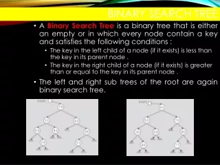
Binary Search Tree Example for for return do while do if while return 3 comparisons in worst case if 4 comparisons in worst case
Extended Binary Tree Example for for return do while do if while return if (b) (a)
External Path Length and Internal Path Length • External path length of a binary tree is the sum over all external nodes of the lengths of the paths from the root to those nodes. • Internal path length is the sum over all internal nodes of the lengths of the paths from the root to those nodes. • Let the internal path length be I and external path length E, then the binary tree of (a) has I = 0+1+1+2+3 = 7, E = 2+2+4+4+3+2 = 17.
External Path Length and Internal Path Length (Cont.) • It can be shown that E = I + 2n. • Binary trees with maximum E also have maximum I. • For all binary trees with n internal nodes, • maximum I = (skew tree) • minimum I = (complete binary tree)
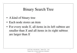
Binary Search Tree Containing A Symbol Table • Let’s look at the problem of representing a symbol table as a binary search tree. If a binary search tree contains the identifiers a1, a2, …, an with a1 < a2 < … < an, and the probability of searching for each ai is pi, then the total cost of any binary search tree is when only successful searches are made.
Binary Search Tree Containing A Symbol Table • For unsuccessful searches, let’s partitioned the identifiers not in the binary search tree into n+1 classes Ei, 0 ≤ i ≤ n. If qi is the probability that the identifier being sought is in Ei, then the cost of the failure node is • Therefore, the total cost of a binary search tree is • An optimal binary search tree for the identifier set a1, …, an is one that minimize the above equation over all possible binary search trees for this identifier set. Since all searches must terminate either successfully or unsuccessfully, we have
Binary Search Tree With Three Identifiers Example do if while if if do while while do (c) (b) while (a) do do while if if (d) (e)
Cost of Binary Search Tree In The Example • With equal probabilities, pi = qj = 1/7 for all i and j, we have cost(tree a) = 15/7; cost(tree b) = 13/7 cost(tree c) = 15/7; cost(tree d) = 15/7 cost(tree e) = 15/7 Tree b is optimal. • With p1=0.5, p2=0.1, p3=0.05, q0=0.15, q1=0.1, q2=0.05, and q3=0.05 we have cost(tree a) = 2.65; cost(tree b) = 1.9 cost(tree c) = 1.5; cost(tree d) = 2.05 cost(tree e) = 1.6 Tree c is optimal.
Determine Optimal Binary Search Tree • So to determine which is the optimal binary search, it is not practical to follow the above brute force approach since the complexity is O(n4n/n3/2). • Now let’s take another approach. Let Tij denote an optimal binary search tree for ai+1, …, aj, i<j. Let cij be the cost of the search tree Tij. Let rij be the root of Tij and let wij be the weight of Tij, where • Therefore, by definition rii=0, wii=qi, 0 ≤ i ≤ n. T0n is an optimal binary search tree for a1, …, an. Its cost function is c0n, it weight w0n, and it root is r0n.
Determine Optimal Binary Search Tree (Cont.) • If Tij is an optimal binary search tree for ai+1, …, aj, and rij=k, then i< k <j. Tij has two subtrees L and R. L contains ai+1, …, ak-1, and R contains ak+1, …, aj. So the cost cij of Tij is cij = pk + cost(L) + cost(R) + weight(L) + weight(R) cij = pk + ci,k-1+ ckj + wi,k-1+ wkj = wij + ci,k-1+ ckj • Since Tij is optimal, we have wij + ci,k-1 + ckj=
Example 10.2 • Let n=4, (a1, a2, a3, a4) = (do, if return, while). Let (p1, p2, p3, p4)=(3,3,1,1) and (q0, q1, q2, q3, q4)=(2,3,1,1,1). wii = qii, cii=0, and rii=0, 0 ≤ i ≤ 4. w01 = p1 + w00 + w11 = p1 +q1 +w00 = 8 c01 = w01 + min{c00 +c11} = 8 r01 = 1 w12 = p2 + w11 + w22 = p2 +q2 +w11 = 7 c12 = w12 + min{c11 +c22} = 7 r12 = 2 w23 = p3 + w22 + w33 = p3 +q3 +w22 = 3 c23 = w23 + min{c22 +c33} = 3 r23 = 3 w34 = p4 + w33 + w44 = p4 +q4 +w33 = 3 c34 = w34 + min{c33 +c44} = 3 r34 = 4
Example 10.2 Computation 2 4 1 3 0 w44=1 c44=0 r44=0 w33=1 c33=0 r33=0 w00=2 c00=0 r00=0 w11=3 c11=0 r11=0 w22=1 c22=0 r22=0 w00=2 c00=0 r00=0 0 w01=8 c01=8 r01=1 w34=3 c34=3 r34=4 w12=7 c12=7 r12=2 w23=3 c23=3 r23=3 1 w02=12 c02=19 r02=1 w13=9 c13=12 r13=2 w24=5 c24=8 r24=3 2 w03=14 c03=25 r03=2 w14=11 c14=19 r14=2 3 w04=16 c04=32 r04=2 4
Computation Complexity of Optimal Binary Search Tree • To evaluate the optimal binary tree we need to compute cij for (j-i)=1, 2, …,n in that order. When j-i=m, there are n-m+1 cij’s to compute. • The computation of each cij’s can be computed in time O(m). • The total time for all cij’s with j-i=m is therefore O(nm-m2). The total time to evaluate all the cij’s and rij’s is • The computing complexity can be reduced to O(n2) by limiting the search of the optimal l to the range of ri,j-1 ≤ l ≤ ri+1,j according to D. E. Knuth.
AVL Trees • Dynamic tables may also be maintained as binary search trees. • Depending on the order of the symbols putting into the table, the resulting binary search trees would be different. Thus the average comparisons for accessing a symbol is different.
Binary Search Tree for The Months of The Year Input Sequence: JAN, FEB, MAR, APR, MAY, JUNE, JULY, AUG, SEPT, OCT, NOV, DEC JAN FEB MAR JUNE MAY APR JULY SEPT AUG DEC OCT Max comparisons: 6 Average comparisons: 3.5 NOV
A Balanced Binary Search Tree For The Months of The Year JAN Input Sequence: JULY, FEB, MAY, AUG, DEC, MAR, OCT, APR, JAN, JUNE, SEPT, NOV Max comparisons: 4 Average comparisons: 3.1 JULY FEB MAY AUG MAR OCT APR DEC JUNE NOV SEPT
Degenerate Binary Search Tree APR AUG Input Sequence: APR, AUG, DEC, FEB, JAN, JULY, JUNE, MAR, MAY, NOV, OCT, SEPT DEC FEB JAN JULY JUNE MAR MAY NOV Max comparisons: 12 Average comparisons: 6.5 OCT SEPT
Minimize The Search Time of Binary Search Tree In Dynamic Situation • From the above three examples, we know that the average and maximum search time will be minimized if the binary search tree is maintained as a complete binary search tree at all times. • However, to achieve this in a dynamic situation, we have to pay a high price to restructure the tree to be a complete binary tree all the time. • In 1962, Adelson-Velskii and Landis introduced a binary tree structure that is balanced with respect to the heights of subtrees. As a result of the balanced nature of this type of tree, dynamic retrievals can be performed in O(log n) time if the tree has n nodes. The resulting tree remains height-balanced. This is called an AVL tree.
AVL Tree • Definition: An empty tree is height-balanced. If T is a nonempty binary tree with TL and TR as its left and right subtrees respectively, then T is height-balanced iff (1) TL and TR are height-balanced, and (2) |hL – hR| ≤ 1 where hL and hR are the heights of TL and TR, respectively. • Definition: The Balance factor, BF(T) , of a node T is a binary tree is defined to be hL – hR, where hL and hR, respectively, are the heights of left and right subtrees of T. For any node T in an AVL tree, BF(T) = -1, 0, or 1.
Balanced Trees Obtained for The Months of The Year -2 0 0 RR MAR MAY MAR -1 0 0 MAY NOV MAR 0 (a) Insert MARCH NOV (c) Insert NOVEMBER -1 +1 MAR MAY 0 0 +1 MAY NOV MAY 0 (b) Insert MAY AUG (d) Insert AUGUST
Balanced Trees Obtained for The Months of The Year (Cont.) +2 +1 MAY LL MAY 0 +2 0 0 NOV MAR NOV AUG +1 0 0 AUG APR MAR 0 (e) Insert APRIL APR 0 +2 MAR MAY -1 0 0 -1 LR MAY NOV AUG AUG 0 0 0 0 +1 NOV APR APR JAN MAR 0 JAN (f) Insert JANUARY
Balanced Trees Obtained for The Months of The Year (Cont.) +1 +1 MAR MAR -1 -1 -1 -1 MAY AUG MAY AUG 0 0 0 0 0 +1 NOV APR JAN NOV APR JAN 0 0 0 JULY DEC DEC (h) Insert JULY (g) Insert DECEMBER
Balanced Trees Obtained for The Months of The Year (Cont.) +2 +1 MAR MAR RL -2 -1 -2 0 MAY MAY AUG DEC 0 0 0 +1 +1 0 NOV NOV APR AUG JAN JAN 0 0 0 -1 0 JULY APR DEC JULY FEB 0 FEB (i) Insert FEBRUARY
Balanced Trees Obtained for The Months of The Year (Cont.) DEC MAY AUG AUG FEB JAN JULY MAY 0 APR FEB +2 MAR 0 LR -1 -1 JAN 0 +1 DEC MAR 0 -1 +1 NOV 0 +1 -1 -1 0 -1 JULY APR 0 0 0 0 NOV JUNE JUNE (j) Insert JUNE
Balanced Trees Obtained for The Months of The Year (Cont.) AUG AUG FEB FEB -1 -1 JAN JAN RR +1 -1 +1 0 DEC MAR DEC MAR -2 -1 +1 0 0 -1 +1 0 JULY MAY JULY NOV 0 0 0 0 0 -1 0 JUNE APR OCT MAY NOV JUNE APR 0 OCT (k) Insert OCTOBER
Balanced Trees Obtained for The Months of The Year (Cont.) DEC MAR AUG FEB JULY NOV -1 JAN -1 +1 -1 -1 0 +1 0 -1 0 0 APR JUNE OCT MAY 0 SEPT (i) Insert SEPTEMBER
Rebalancing Rotation of Binary Search Tree • LL: new node Y is inserted in the left subtree of the left subtree of A • LR: Y is inserted in the right subtree of the left subtree of A • RR: Y is inserted in the right subtree of the right subtree of A • RL: Y is inserted in the left subtree of the right subtree of A. • If a height–balanced binary tree becomes unbalanced as a result of an insertion, then these are the only four cases possible for rebalancing.
Rebalancing Rotation LL LL +1 A +2 A 0 B 0 B BL 0 A +1 B AR AR h+2 h+2 h BL BR BL BR BR AR height of BL increases to h+1
Rebalancing Rotation RR RR -1 A -2 A 0 B 0 B 0 A BR -1 B AL AL h+2 h+2 BR BL BR BL AL BL height of BR increases to h+1
Rebalancing Rotation LR(a) +1 A +2 A 0 C LR(a) 0 B -1 B 0 B 0 A 0 C
Rebalancing Rotation LR(b) 0 B -1 A CR CR LR(b) +1 A +2 A 0 C 0 B -1 B AR AR h+2 h+2 0 C +1 C h BL BL h BL AR CR CL CL CL h
Rebalancing Rotation LR(c) +1 B 0 A CR 0 C +2 A LR(c) -1 B AR h+2 -1 C BL BL AR CR CL h CL
AVL Trees (Cont.) • Once rebalancing has been carried out on the subtree in question, examining the remaining tree is unnecessary. • To perform insertion, binary search tree with n nodes could have O(n) in worst case. But for AVL, the insertion time is O(log n).
AVL Insertion Complexity • Let Nh be the minimum number of nodes in a height-balanced tree of height h. In the worst case, the height of one of the subtrees will be h-1 and that of the other h-2. Both subtrees must also be height balanced. Nh = Nh-1 + Nh-2 + 1, and N0= 0, N1 = 1, and N2 = 2. • The recursive definition for Nh and that for the Fibonacci numbers Fn= Fn-1 + Fn-2, F0=0, F1= 1. • It can be shown that Nh= Fh+2 – 1. Therefore we can derive that . So the worst-case insertion time for a height-balanced tree with n nodes is O(log n).
Probability of Each Type of Rebalancing Rotation • Research has shown that a random insertion requires no rebalancing, a rebalancing rotation of type LL or RR, and a rebalancing rotation of type LR and RL, with probabilities 0.5349, 0.2327, and 0.2324, respectively.
Comparison of Various Structures • Doubly linked list and position of x known. • Position for insertion known
2-3 Trees • If search trees of degree greater than 2 is used, we’ll have simpler insertion and deletion algorithms than those of AVL trees. The algorithms’ complexity is still O(log n). • Definition: A 2-3 tree is a search tree that either is empty or satisfies the following properties: (1) Each internal ndoe is a 2-node or a 3-node. A 2-node has one element; a 3-node has two elements. (2) Let LeftChild and MiddleChild denote the children of a 2-node. Let dataL be the element in this node, and let dataL.key be its key. All elements in the 2-3 subtree with root LeftChild have key less than dataL.key, whereas all elements in the 2-3 subtree with root MiddleChild have key greater than dataL.key. (3) Let LeftChild, MiddleChild, and RightChild denote the children of a 3-node. Let dataL and dataR be the two elements in this node. Then, dataL.key < dataR.key; all keys in the 2-3 subtree with root LeftChild are less than dataL.key; all keys in the 2-3 subtree with root MiddleChild are less than dataR.key and greater than dataL.key; and all keys in the 2-3 subtree with root RightChild are greater than dataR.key. (4) All external nodes are at the same level.
2-3 Tree Example A 40 B C 10 20 80
The Height of A 2-3 Tree • Like leftist tree, external nodes are introduced only to make it easier to define and talk about 2-3 trees. External nodes are not physically represented inside a computer. • The number of elements in a 2-3 tree with height h is between 2h - 1 and 3h - 1. Hence, the height of a 2-3 tree with n elements is between and
2-3 Tree Data Structure template<class KeyType> class Two3; class Two3Node { friendclass Two3<KeyType>; private: Element<KeyType> dataL, dataR; Two3Node *LeftChild, *MiddleChild, *RightChild; }; template<class KeyType> class Two3{ public: Two3(KeyType max, Two3Node<KeyType>* int=0) : MAXKEY(max), root(init) {}; // constructor Boolean Insert(const Element<KeyType>&); Boolean Delete(const Element<KeyType>&); Two3Node<KeyType>* Search(const Element<KeyType>&); private: Two3Node<KeyType>* root; KeyType MAXKEY; };
Searching A 2-3 Tree • The search algorithm for binary search tree can be easily extended to obtain the search function of a 2-3 tree (Two3::Search()). • The search function calls a function compare that compares a key x with the keys in a given node p. It returns the value 1, 2, 3, or 4, depending on whether x is less than the first key, between the first key and the second key, greater than the second key, or equal to one of the keys in node p.
Searching Function of a 2-3 Tree template <class KeyType> Two3Node<KeyType>* Two3<KeyType>:: Search(const Element<KeyType>& x) // Search the 2-3 tree for an element x. If the element is not in the tree, then return 0. // Otherwise, return a pointer to the node that contains this element. { for (Two3Node<KeyType>* p = root; p;) switch(p->compare(x)){ case 1: p = p->LeftChild; break; case 2: p = p->MiddleChild; break; case 3: p = p->RightChild; break; case 4: return p; // x is one of the keys in p } }
Insertion Into A 2-3 Tree • First we use search function to search the 2-3 tree for the key that is to be inserted. • If the key being searched is already in the tree, then the insertion fails, as all keys in a 2-3 tree are distinct. Otherwise, we will encounter a unique leaf node U. The node U may be in two states: • the node U only has one element: then the key can be inserted in this node. • the node U already contains two elements: A new node is created. The newly created node will contain the element with the largest key from among the two elements initially in p and the element x. The element with the smallest key will be in the original node, and the element with median key, together with a pointer to the newly created node, will be inserted into the parent of U.
Insertion to A 2-3 Tree Example A A 20 40 40 C B D B C 70 80 10 30 10 20 70 80 (b) 30 inserted (a) 70 inserted
Insertion of 60 Into Figure 10.15(b) 60 80 10 30 G 40 A F 20 70 E B D C
Node Split • From the above examples, we find that each time an attempt is made to add an element into a 3-node p, a new node q is created. This is referred to as a node split.
2-3 Tree Insertion Function template <class KeyType> Boolean Two3<KeyType>::Insert(const Element<KeyType>& y) { Two3Node<KeyType>* p; Element<KeyType> x = y; if (x.key>=MAXKEY) return FALSE; // invalid key if (!root) {NewRoot(x, 0); return TRUE;} if (!(p = FindNode(x))){ InsertionError(); return FALSE;} for (Two3Node<KeyType> *a = 0;;) if (p->dataR.key == MAXKEY) { // p is a 2-node p->PutIn(x, a); return TRUE; } else { // p is a 3-node Two3Node<KeyType>* olda = a; a = new(Two3Node<KeyType>); x = Split(p, x, olda, a); if (root == p) { // root has been split NewRoot(x, a); return TRUE; } else p = p->parent(); } }
Deletion From a 2-3 Tree • If the element to be deleted is not in a leaf node, the deletion operation can be transformed to a leaf node. The deleted element can be replaced by either the element with the largest key on the left or the element with the smallest key on the right subtree. • Now we can focus on the deletion on a leaf node.
Deletion From A 2-3Tree Example A A 50 80 50 80 B C D B C D 90 95 10 20 60 90 95 10 20 60 70 (b) 70 deleted A (a) Initial 2-3 tree 50 80 B C D 95 10 20 60 (c) 90 deleted