Binary Search Trees: Operations and Traversals
Learn about Binary Search Tree (BST) operations like insertion, deletion, and searching. Explore tree traversals including Preorder, Inorder, and Postorder. Understand the algorithms with helpful examples.

Binary Search Trees: Operations and Traversals
E N D
Presentation Transcript
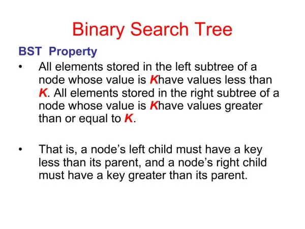
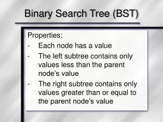
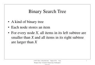
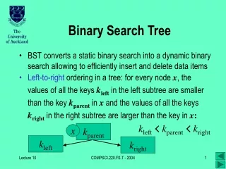
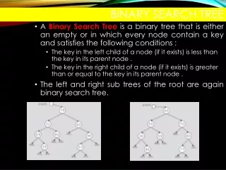
Arbitrary binary tree Binary search tree Binary Search Tree • A Binary Search Treeis a binary tree that is either an empty or in which every node contain a key and satisfies the following conditions : • The key in the left child of a node (if it exists) is less than the key in its parent node . • The key in the right child of a node (if it exists) is greater than or equal to the key in its parent node . • The left and right sub trees of the root are again binary search tree.
Binary Search Tree (ADT) ADT Implementation of BST: struct BSTNode { int data; BSTNode *left; BSTNode *right; } struct BSTnode*left=NULL ,*right=NULL; BSTs can be implemented using either arrays or linked lists. However, linked list structures are more common and more efficient. The implementation uses nodes with two pointers namely, left and right.
Binary Search Tree (ADT) A BST implementation
Operations- Traversal, Searching, Insertion and Deletion • There are four basic BST operations: traversal, search, insert, and delete. • Traversals: Traverse the items in a binary search tree in preorder, inorder, or postorder • Searches: Retrieve the item with a given search key from a binary search tree • Insertion: Insert a new item into a binary search tree • Deletion Delete the item with a given search key from a binary search tree
Traversals Traversals:Traverse the items in a binary search tree in preorder, inorder, or postorder • There are 3 types of traversals: • 1. Pre-Order • 2. In-Order • 3. Post-Order
Inorder Traversal To traverse a non-empty binary tree using in order, perform the following operations recursively at each node, starting with the root node: • Traverse the left sub tree. • Visit the root. • Traverse the right sub tree. Visit the nodes in the left subtree, then visit the root of the tree, then visit the nodes in the right subtree • Inorder(tree) • If tree is not NULL • Inorder(Left(tree)) • Visit Info(tree) • Inorder(Right(tree)) • ("visit" means that the algorithm does something with the values in the node, e.g., printthevalue)
‘J’ Inorder Traversal : A E H J M T Y Visit second tree ‘T’ ‘E’ ‘A’ ‘H’ ‘M’ ‘Y’ Visit left subtree first Visit right subtree last
Preorder Traversal • To traverse a non-empty binary tree in preorder, perform the following operations recursively at each node, starting with the root node: • Visit the root. • Traverse the left sub tree. • Traverse the right sub tree. • Visit the root of the tree first, then visit the nodes in the left subtree, then visit the nodes in the right subtree Preorder(tree) If tree is not NULL Visit Info(tree) Preorder(Left(tree)) Preorder(Right(tree))
‘J’ Preorder Traversal: J E A H T M Y Visit first tree ‘T’ ‘E’ ‘A’ ‘H’ ‘M’ ‘Y’ Visit left subtree second Visit right subtree last
Postorder Traversal • To traverse a non-empty binary tree in post order, perform the following operations recursively at each node, starting with the root node: • Traverse the left sub tree. • Traverse the right sub tree. • Visit the root. • Visit the nodes in the left subtree first, then visit the nodes in the right subtree, then visit the root of the tree Postorder(tree) If tree is not NULL Postorder(Left(tree)) Postorder(Right(tree)) Visit Info(tree)
‘J’ Visit last tree ‘T’ ‘E’ ‘A’ ‘H’ ‘M’ ‘Y’ Visit left subtree first Visit right subtree second Postorder Traversal: A H E M Y T J
SEARCH Searches: Retrieve the item with a given search key from a binary search tree. Three BST search algorithms: Find the smallest node Find the largest node Find a requested node
BST INSERTION • To insert data, all we need to do is follow the branches to an empty sub tree and then insert the new node. • In other words, all inserts take place at a leaf or at a leaf like node – a node that has only one null sub tree.
Algorithm addBST (root, newNode) Insert node containing new data into BST using recursion . Pre root is address of current node in a BST newNode is address of node containing data Post neewNode inserted into the tree Return address of potential new tree root if (empty tree) set root to newNode return newNode end if Locate null subtree for insertion if(newNode<root) return addBST(left subtree,newNode) else return addBST(right subtree, newNode) end if end addBST
Deletion The following possible cases are expected during a node deletion: • The node to be deleted has no children. In this case, all we need to do is delete the node. • The node to be deleted has only a right sub tree. We delete the node and attach the right sub tree to the deleted node’s parent. • The node to be deleted has only a left sub tree. We delete the node and attach the left sub tree to the deleted node’s parent. • The node to be deleted has two sub trees. It is possible to delete a node from the middle of a tree, but the result tends to create very unbalanced trees.
Deletion from the middle of a tree: • Rather than simply delete the node, we try to maintain the existing structure as much as possible by finding data to take the place of the deleted data. This can be done in one of the two ways. • We can find the largest node in the deleted node’s left subtree and move its data to replace the deleted node’s data. • We can find the smallest node on the deleted node’s right subtree and move its data to replace the deleted node’s data. • Either of these moves preserves the integrity of the binary search tree.
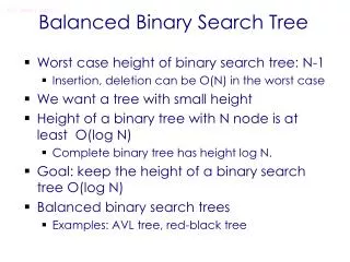
AVL TREES • Definition: balanced tree is a binary search tree, which is either (a) empty or (b) its left and right sub-trees are “more or less” of equal height • Definition: AVL (Adelson-Velski, Landis) tree is a binary search tree T, which is either (a) empty or (b) difference between heights of its left and right sub-trees is not greater than one and both sub-trees are also AVL trees • |hleft-hright| <=1 • A tree is said to be balanced if for each node, the number of nodes in the left subtree and the number of nodes in the right subtree differ by at most one.
Height of an AVL TREE • A tree is said to be height-balanced or AVL if for each node, the height of the left subtree and height of the right subtree differ by at most one. • The height of the left subtree minus the height of the right subtree of a node is called the balance of the node. For an AVL tree, the balances of the nodes are always -1, 0 or 1. • Given an AVL tree, if insertions or deletions are performed, the AVL tree may not remain height balanced.
-1 10 1 1 7 40 0 0 1 -1 3 8 30 45 0 0 0 -1 0 1 5 20 35 60 0 25 AVL Tree with Balance Factors
AVL TREES SEARCH • To search an AVL search tree, the code for searching a binary search tree can be used without any change
Rebalancing Suppose the node to be rebalanced is X. There are 4 cases that we might have to fix (two are the mirror images of the other two): • An insertion in the left subtree of the left child of X, • An insertion in the right subtree of the left child of X, • An insertion in the left subtree of the right child of X, or • An insertion in the right subtree of the right child of X. Balance is restored by tree rotations.
Single Rotation • A single rotation switches the roles of the parent and child while maintaining the search order. • Single rotation handles the outside cases (i.e. 1 and 4). • We rotate between a node and its child. • Child becomes parent. Parent becomes right child in case 1, left child in case 4. • The result is a binary search tree that satisfies the AVL property.
Double Rotation • Single rotation does not fix the inside cases (2 and 3). • These cases require a double rotation, involving three nodes and four subtrees.
Left–right double rotation to fix case 2 Lift this up: first rotate left between (k1,k2), then rotate right betwen (k3,k2)
Left-Right Double Rotation • A left-right double rotation is equivalent to a sequence of two single rotations: • 1st rotation on the original tree: a left rotation between X’s left-child and grandchild • 2nd rotation on the new tree: a right rotation between X and its new left child.
AVL TREE INSERTION • First search the tree and find the place where the new item is to be inserted • Can search using algorithm similar to search algorithm designed for binary search trees • If the item is already in tree • Search ends at a nonempty subtree • Duplicates are not allowed • If item is not in AVL tree • Search ends at an empty subtree; insert the item there • After inserting new item in the tree • Resulting tree might not be an AVL tree
AVL tree before and after inserting 90 AVL tree before and after inserting 75
AVL tree before and after inserting 95 AVL tree before and after inserting 88
2 2 3 2 3 4 4 1 1 1 2 2 3 3 Fig 1 5 3 3 Fig 4 Fig 2 Fig 3 1 Fig 5 Fig 6 Example Insert 3,2,1,4,5,6,7, 16,15,14