Download

1 / 29
290 likes | 311 Vues
Simplify complex numbers, factor polynomials, and graph polynomial functions with real and non-real zeros. Understand the end behavior, leading coefficient, degree, and number of real and non-real zeros.

E N D
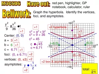
total: pencil, red pen, highlighter, GP notebook U7D8 Have out: Bellwork: 1. Simplify the complex numbers. Write part (b) in a + bi form. +1 +1 a) b) r 3 16 2. Factor p(x) = x3 – 64, then find all zeros.
total: 1. Simplify, and write in a + bi form. 2. Factor p(x) = x3 – 64, then find all zeros. +1 b) +2 find the zeros: +1 +1 4 4 +1 +1 +1 +1 +1 +1 +1
y y y x x x conjugate Complex zeros always come in __________ pairs. 0 2 A cubic polynomial could have ___ or ___ complex zeros, and ___, ___, or ___ real zeros. 3 1 2 possibilities: 1 real 2 real (one is double) 3 real 0 non–real 0 non–real 2 non–real
y y y y x x x x y x 0 2 4 A fourth degree polynomial could have ___, ___, or ___ complex zeros, and ___, ___, ___, ___, or ___ real zeros. 0 1 2 3 4 possibilities: 0 real 1 real (but it’s double) 2 real 4 non–real 2 non–real 2 non–real 3 real, but one is double 4 real 0 non–real 0 non–real
REMEMBER: conjugate pair When there is a complex zero there is always a _____________.
y x Turning Points to Degree Principle direction Turning points ____________ – points where the graph changes _________ from increasing to decreasing or decreasing to increasing. n–degree An _________ polynomial function has at most _____ turning points. n – 1 2 For example, a 4th degree polynomial has at most 3 turning points. However in many other cases, it is possible to have less. 3 1 n Using the same principle, a polynomial that has ___ turning points has a degree of ______ or greater. n + 1
P(x) x 2. For each graph, a) describe the end behavior and describe the leading coefficient (+ / –) b) determine whether it represents an odd-degree or an even-degree polynomial function, and guess it’s minimum value. c) state the number of real zeros. d) state the number of non-real values. 1 End behavior: Leading coefficient: Degree: Real zeros: Non–real zeros: a) + odd, 3 3 0 2 To compute the minimum degree, count the number of turning points, then add 1. The real zeros are the ones where the graph crosses the x–axis. Remember: real + non-real = degree
P(x) x b) End behavior: Leading coefficient: Degree: Real zeros: Non–real zeros: 2 + even, 4 4 0 3 To compute the minimum degree, count the number of turning points, then add 1. 1 P(x) End behavior: Leading coefficient: Degree: Real zeros: Non–real zeros: c) – even, 4 1 3 0 x 4 How may zeros are left? 2 Try the next few on your own...
P(x) x d) e) P(x) x End behavior: Leading coefficient: Degree: Real zeros: Non–real zeros: End behavior: Leading coefficient: Degree: Real zeros: Non–real zeros: + + odd, 5 odd, 3 5 1 0 2 Remember: real + non-real = degree
g) f) P(x) P(x) x x End behavior: Leading coefficient: Degree: Real zeros: Non–real zeros: End behavior: Leading coefficient: Degree: Real zeros: Non–real zeros: – – even, 6 odd, 9 2 1 4 8
h) P(x) double zero! End behavior: Leading coefficient: Degree: Real zeros: Non–real zeros: x + even, 6 3 2
Get out the worksheet: Graphing Polynomial Functions With Non–Real Zeros Part 1: Determine the degree and zeros. Sketch a graph of the polynomial function. 3 1) 3, ±2i When we graph this function, can we graph all the zeros (real and non–real)? No! We can only graph the real zeros on a Cartesian plane.
y x 3 1) 3, ±2i Graph the only real x–intercept. Next thing to consider: how do we graph the function and still make it look like a 3rd degree polynomial? (3, 0) We must have an inflection point some–where on the graph because it is cubic. Graph the y–intercept Therefore, we only know 4 things: (0, –12) (1) x–intercept (2) y–intercept (3) end behavior (4) inflection point is somewhere However, we don’t know the effect of the non–real zeros on the polynomial.
y x 3 1) 3, ±2i We only know 4 things: (1) x–intercept (2) y–intercept (3, 0) (3) end behavior (4) inflection point is somewhere There are several acceptable graphs that meet these 4 criteria. (0, –12) Draw your graph. Be careful to cross the x–axis only once through the real zero, and make sure that the graph passes the vertical line test.
y x 3 1) 3, ±2i The actual graph is given on the left. Does your graph look like this? Maybe not, but that’s okay. (3, 0) Since we are NOT using graphing calculators, we have some freedom when we sketch graphs. Therefore, there are many acceptable answers. (0, –12) Let’s look at some other possibilities…
y y (3, 0) x x (0, –12) 3 1) 3, ±2i (3, 0) (0, –12) All of these graphs meet the 4 criteria. Any other possibilities out there?
2) 4 x = ±3, ± 3i y non–real solutions 2 real (–3, 0) (3, 0) x We can ONLY graph the real zeros. (0, –81)
2) 4 x = ±3, ± 3i What are the criteria we know? y (1) x–intercept (2) y–intercept (3) end behavior (–3, 0) (3, 0) x Draw a 4th degree polynomial that fits these criteria. (0, –81) Does your graph look like this? No? Let’s look at other possibilities…
y (–3, 0) (3, 0) x (0, –81) 2) 4 x = ±3, ± 3i y (–3, 0) (3, 0) x (0, –81) Even though these are not the correct graph, they are acceptable at this point in Algebra 2 without a graphing calculator. You will have to wait until Math Analysis for further details.
3 3) x = 0, ±5i y x (0, 0) There is only one real zero and 2 non–real zeros. Only graph the real zero.
3 3) x = 0, ±5i We only know 4 things: y (1) x–intercept (2) y–intercept (same as x–int) (3) end behavior (4) inflection point is somewhere since the function is cubic x (0, 0) Draw a 3rd degree polynomial that fits these criteria. Does your graph look like this? Let’s look at other possibilities…
3 3) x = 0, ±5i y y x x (0, 0) (0, 0) All of these graphs meet the 4 criteria. Any other possibilities out there?
–3 –2 4 4) y –3 1 x (0, –3) There are 2 real zeros and 2 non–real zeros. Only graph the real zeros.
4 4) What are the criteria we know? y (1) x–intercept (2) y–intercept (3) end behavior x Draw a 4th degree polynomial that fits these criteria. (0, –3) Does your graph look like this? Let’s look at other possibilities…
4 4) y y x x (0, –3) (0, –3) All of these graphs meet the criteria. Any other possibilities out there?
(–2, 4) Day 7 Mixed Practice 1a) Determine the function that generates each graph below. roots: x = –4, 0, 2 Double zero P(x) = a (x + 4) (x)2 (x – 2 ) 4 = a(–2+4)(–2)2(–2 – 2) Boing! 4 = a(2)(4)(–4) 4 = a(–32)
Day 7 Mixed Practice 1d) Determine the function that generates each graph below. zeros: x = –2, 1, 3 P(x) = a (x + 2)3 (x – 1) (x – 3)2 –2 = a(–1+2)3(–1 – 1)(–1 – 3)2 –2 = a(1)3(–2)(–4)2 (–1, –2) Double zero (squared term) –2 = a(–2)(16) –2 = a(–32) triple zero (cubic term)
3. Simplify. a) b) c)