Gold Returns
Gold Returns. Robert J. Barro Sanjay Misra. Gold. Gold has dominated monetary systems for centuries ; plays prominent role in transactions among financial institutions even in modern systems with fiat money.

Gold Returns
E N D
Presentation Transcript
Gold Returns Robert J. Barro Sanjay Misra
Gold • Gold has dominated monetary systems for centuries;plays prominent role in transactions among financial institutions even in modern systems with fiat money. • Private holdings of gold important, facilitated in recent years by availability of liquid futures contracts on commodity exchanges. • Gold often viewed as hedge against disaster scenarios, but risk premium on gold not well understood. We study determinants of this risk premium.
Baseline Model of Returns on Gold with Rare Disasters • Underlying demand for gold reflects service value proportional to stock of gold. • Matches with gold used as jewelry, etc. • Gold also provides monetary services—transactions and liquid store-of-value benefit considered in analyses of demand for money. Special physical characteristics of gold. • Monetary role central in world gold standard.
Gold as Jewelry or Money • Important difference in two approaches: jewelry relates to gold in physical units; monetary services to gold in units of value in terms of other goods. That is, relative price of gold and other goods enters into monetary service flow and, hence, household utility (as in Sidrauski). • Initial model treats gold as jewelry, and extension considers monetary services.
Baseline Model • Use “two-tree” version of Lucas-tree model to consider evolution of ordinary consumption, ct, and gold, gt. • Specification closest to model of Piazzesi, Schneider, and Tuzel (2007), in which second tree corresponds to residential housing. In their model, variations in share of consumer expenditure directed to housing have important implications for asset pricing. • In contrast, we assume (reasonably) that fraction of total consumer outlay directed to gold services always negligible; therefore, do not get these types of effects.
Ordinary consumption and gold services imperfect substitutes in effective consumption flow for representative consumer; constant elasticity of substitution, σ. • Outlay on gold services negligible compared to ordinary consumption. • Disaster and other shocks apply directly to ordinary consumption (and GDP), not gold.
Representative household’s utility depends on effective consumption flow, which relates to ordinary consumption, ct, and flow of services from gold stock, gt, in CES form: (1) σ>0, 0<αt<1.
Rental price, > 0, for gold equals ratio of marginal utility of gold services to marginal utility of ordinary consumption: (2) • Gold relatively highly valued when ct/gthigh and αtlow. Rental price determines dividend for holders of gold. Assume initially that αt equals constant, α.
Lucas Tree for Consumption • Stochastic process for ct, viewed as fruit from Lucas tree, takes same form as Barro (2006): (4) log(ct+1) = log(ct) + h + ut+1 + vt+1 • h≥0 is exogenous productivity growth, ut+1 is i.i.d. normal shock with mean 0, variance . Number of trees fixed, no loss of ownership, economy closed.
vt+1 is disaster shock, governed by constant Poisson arrival probability p≥0 and proportionate disaster size, b≥0, subject to time-invariant probability distribution. • Expected growth rate, h*, of ct: (5)
Pt is price of unlevered equity claim on tree. Gross, one-period return on tree equity is: (6) • Utility time-additive, depends on in usual iso-elastic way with coefficient of relative risk aversion γ>0 and time-preference rate ρ≥0. (E-Z preferences okay with i.i.d. shocks.) • Simplifying assumption is that preference parameter, α, and per capita quantities of gold, gt, and consumption, ct, such that outlay on gold services negligible compared to ct.
First-order condition for choosing ct over time and holding assets as equity claims on trees: (7) Because of i.i.d. shocks, ratio of consumption dividend to equity price, ct/Pt, approximately constant in equilibrium.
Define re to be expectation of rate of return on equity, Rt -1. Solution is: (9) • Risk-free rate: (10)
Equity premium: (11) • Pricing of gold: (13)
Gold Stock • Per capita gold stock, gt, grows deterministically at constant rate, hg. • Estimate hgbased on long-run growth rate of per capita world stock of gold. Results in Figure 1 imply long-run growth rate (1875 to 2011) between 0.4% and 0.9% per year if we neglect loss or depreciation of gold stock.
As with tree equity, dividend-price ratio for gold, denoted χ, constant in this i.i.d. model. Constancy of this ratio means that real gold price, , moves along with . • In model, positive valuation of gold depends on intrinsic usefulness—equilibrium does not allow gold to have positive value based on process for real price unlinked to underlying service value.
Rate of Return on Gold ] • Define rg to be expectation of rate of return on gold, -1. Solution: (15) • Compared to return on equity, result is: (16)
Compared to risk-free rate, result is: (17) • Comparison of gold return with others depends on σ, elasticity of substitution between gold services and ordinary consumption in effective consumption flow. When σ=1, returns on gold mimic returns on tree equity, so re-rg= 0 in (16). As σ approaches infinity, rental price of gold becomes unresponsive to ct/gt, and gold becomes risk-free. Therefore, rg- rf = 0 in (17). • Depending on value of σ in range where σ≥1, rg ranges between re and rf. Thus, given measure of rg—assuming it lies between rf and re—there is σ>1 that makes that observation consistent with model.
In baseline model—with demand for gold derived from role in effective consumption—there is no σ>0 that generates rgbelow rf. That is, gold never enough of a disaster hedge so that risk premium negative. • Particular pattern of shocks to preferences, αt, may generate rg<rf. However, since empirical covariance between consumption growth and growth rate of real gold price turns out to be negligible, unclear that one wants a model with rg<rf.
Shocks to Preferences • Shocks to preferences, αt. Main result is to help explain observed volatility of real gold prices. Volatility depends on nature of monetary regime, including prospects for moving on or off gold standard. • Shocks to stock of gold can be added. Some of supply response buffers effects of shocks to preferences.
Monetary Demand for Gold • Expand effective consumption to include monetary services from real quantity of gold held as “money” (as in Sidrauski). Includes holdings of official gold reserves by central banks & governments. • Shifts in monetary demand are another source of volatility of real gold prices (more important than shifts in demand for jewelry).
Equilibrium not Pareto optimal because of presence of relative price, , in effective consumption flow. • Equilibrium with positive real gold price exists and is unique (given constraint that only gold used as “money”). Gold valued even if no value as jewelry. Real money balances independent of world stock of gold.
Official gold reserves important part of world stock of gold. Figure 2 shows that share of world’s gold stock held as official reserves less than 10% in 1877 but rose to peak of 50-60% at end of WWII in 1945. Share fell to 20% in 2011. • Need to expand data on official reserves and include gold held as coins, etc.
Calibration of Model • Use these parameters (based on previous studies of rare macro disasters): • rf = 0.011 per year, • re = 0.059 per year, • h = 0.025 per year, • hg=0, • σu = 0.02 per year, • p = 0.037 per year, • γ = 3.34, • ρ=0.027 per year, • Eb = 0.208, • E(1-b)-γ = 3.62, • E(1-b)1-γ = 2.16
Missing Data on Dividends • Big effect on mean real rate of return, e.g. on stocks, as is well known. • As period length becomes negligible, no effect on measures of volatility and covariance. • This works for data on stock returns!
As discussed later, mean growth rate of real gold prices from 1836 to 2011 is 1.1% per year. In model (given calibration parameters), expected rate of real price change for gold equals 1.1% if σ=1.5. • Correspondingly, rgis 4.7% and unobserved dividend yield on gold is 3.6% (77% of total return).
Problem is that s.d. of observed growth rate of real gold prices is 13.1% per year, which corresponds to s.d. for mean over 176 years of 1.0% per year. Therefore, one-s.d. confidence interval for mean growth rate of real gold prices is roughly (0.1%, 2.1%). • Range corresponds to interval for estimated σ in calibrated model from 16 to 0.84. Correspondingly, rg ranges from 1.6% to 6.4%, and share of dividend varies from 94% to 67%. • Hence, this method by itself does not pin down unobserved dividend yield on gold and, thereby, rg. Later bring in additional information related to observed covariance between changes in real gold prices and consumption growth
Table 2: Covariances [Correlations] of Real Asset Returns with Consumption Growth Rates
Table 3: Covariances [Correlations] of Real Gold Returns with other Real Asset Returns
Figure 4Real Gold Price, annual average, 1800-2011U.S. dollar price, divided by U.S. CPI
Mean Returns • Over full sample, 1836‑2011, mean real rates of price change on gold and silver similar—1.1% and 1.2% per year, cols. 2 and 3 of Table 1. • Mean real stock return for 1836-2011 is 7.4% (col. 4). • Since available proxies for returns on short-term U.S. government securities (“T-Bills”) up to 1919 unreliable, focus on mean real rate of return, 1.0%, for 1920-2011 (col. 5). • Longer-term U.S. govt. bonds (roughly 10-year maturity), mean real rate of return for 1836-2011 is 2.9% (col. 6).
Volatilities • s.d. of T-Bill return smallest among assets considered—4.3% from 1920 to 2011. • s.d. of real stock returns from 1836 to 2011 is high, 16.1% per year. Means and s.d.’s of real stock returns reasonably stable over sub-periods and well above those on T-Bills and govt. bonds.
Empirical Gold Returns • For 1836‑2011, s.d.’s of real rates of price change for gold and silver, 13.1% and 17.9%, similar to stocks. However, s.d.’s depend on sub-period. • For example, s.d. of real rate of price change for gold for 1880-1913 (peak of world gold standard; see Figure 3) only 2.6%, whereas that for 1975-2011 is 20.7%, higher than for stocks.
Covariances of Returnswith consumption and GDP growth rates 1920-2011: sample covariance of real T-Bill return with growth rate of real per capita consumption (personal consumer expenditure) essentially zero (Table 3, col. 5). Hence, with γ around 4, real bill return of 1.0% (1920-2011) should be close to risk-free rate.
Stock Returns • Real stock return clearly procyclical, gauged by covariances with consumption or GDP growth rates over various sub-periods (Table 2, col. 4). • For 1836-2011, sample covariance with consumption growth is 0.0022 (correlation of 0.36), statistically significantly different from zero. • Note timing—stock returns based on annual averages.
Gold Returns • Mean real rate of price change for gold 1836-2011 (Table 1, col. 2) 1.1%, s.d. 13.1%. • In contrast, during high point of world gold standard (1880-1913), average real rate of price change slightly negative, -1.0%, with small s.d., 2.6%. Since nominal gold price essentially constant (Figure 3), patterns reflect inflation (Table 1, col. 6).
Gold Regimes • In first sub-period, 1836-1879, U.S. (or U.K.) monetary system linked to silver or gold for much of sample (bimetallism), but suspension of monetary convertibility near beginning of U.S. Civil War in 1861; full convertibility in 1879 (Figure 3). • 1914-1974, U.S. maintained aspects of gold standard, but rise in nominal gold price and prohibition of private holdings of monetary gold in 1933 (Figure 3). • In 1971, U.S. formally dropped commitment to foreign central banks to convert U.S. dollars into gold at fixed dollar price. At beginning of 1975, prohibition on private holdings of monetary gold in U.S. lifted. In recent sub-period, 1975-2011, gold retained commodity-reserve role for central banks but one largely divorced from domestic monetary systems.
Suspensions & Resumptions • Table 1, col. 2 shows that mean and s.d. of gold’s real rate of price change vary substantially across sub-periods. However, focusing on period such as 1880-1913—high point of international gold standard—involves strong element of ex post selection. Ex ante, 1880-1913 shares with preceding and subsequent periods possibility of moving off gold standard in certain circumstances, particularly associated with war. Examples are U.S. movement off gold/silver commodity standard in 1861 during Civil War, movements of many countries off gold at start of WWI in 1914, and, much earlier, British movement off gold in 1797 during wars with France. • At times of suspension, important issue was prospect of eventual return to gold or gold/silver standard, likely during peacetime, and at what parity. British resumption of gold standard in 1821 was at old parity (urged by David Ricardo), as was U.S. resumption in 1879 (Figure 3). However, British return to gold in 1925 at previous parity unsuccessful in wake of Great Depression.
Gold: 1975-2011 Compared with history, 1975-2011 shows much higher mean and s.d. of real rate of price change for gold—4.0% and 20.7%, respectively. Although increase in volatility clear, change in mean less sure because hard to pin down when volatility this high. If annual s.d. known to be 20.7%, s.d. of mean over 37 years is 3.4%. Hence, mean real rate of price change of 4.0% not statistically significantly different from zero.
Implications for Gold • Given last perspective and sample-selection issues, seems best to focus on statistics for gold over full sample, 1836-2011. Key points from Tables 1 and 2 are mean real rate of price change of 1.1% per year, s.d. 13.1%, covariance with consumption growth essentially zero, -0.0002 (correlation ‑0.05). • With coefficient of relative risk aversion, γ, around 4, rg should be close to rf , around 1.0%.
In baseline model, need high σ to accord with negligible covariance between gold’s real rate of price change and consumption growth. • Combine this observation with finding from before that long-term sample mean of gold’s real rate of price change—1.1% per year, with one-s.d. confidence interval of roughly (0.1%, 2.1%)—corresponded in baseline model to range for σ from 16 to 0.84. Low values of σ within this range inconsistent with rg being close to rf. For example, σ=1 implies rg = 5.9% (same as re), and σ=2 implies rg =4.0%.
High end of range for σ produces more satisfactory results. σ=10 generates rg=1.8%, with expected rate of change of real gold prices of 0.2%; σ=16 generates rg=1.6%, with expected rate of change of real gold prices of 0.1%. Hence, high values of σ generate values of rgonly small amounts above rf, while also producing expected rates of change of real gold prices within one-s.d. band for long-run mean, (0.1%, 2.1%). • Notable feature of results is that bulk of rg comes from unobserved dividend yield, with only small part reflecting expected real rate of price change.
Extensions • One useful extension would consider gold as tradable good in world of open economies. Framework would include tradable consumer goods and non-tradable goods consumed within each country. • Risk characteristics of gold from perspective of each country depend on quantity of world tradables and on country variables that determine real exchange rate, in sense of relative price of non-tradable home goods and tradable goods, including gold.

