Download

1 / 25
250 likes | 376 Vues
Measurements. Meir Kalech Partially Based on slides of Brian Williams and Peter struss. Outline. Last lecture: Justification-based TMS Assumption-based TMS Consistency-based diagnosis Today’s lecture: Generation of tests/probes Measurement Selection Probabilities of Diagnoses.

E N D
Measurements Meir Kalech Partially Based on slides of Brian Williams and Peter struss
Outline • Last lecture: • Justification-based TMS • Assumption-based TMS Consistency-based diagnosis • Today’s lecture: • Generation of tests/probes • Measurement Selection • Probabilities of Diagnoses
Generation of tests/probes • Test: test vector that can be applied to the system • assumption: the behavior of the component does not change between tests • approaches to select the test that can discriminate between faults of different components (e.g. [Williams]) • Probe: selection of the probe based on: • predictions generated by each candidate on unknown measurable points • cost/risk/benefits of the different tests/probes • fault probability of the various components
Generation of tests/probes (II) Approach based on entropy [deKleer, 87, 92] • A-priori probability of the faults (even a rough estimate) • Given set D1, D2, ... Dn of candidates to be discriminated • Generate predictions from each candidate • For each probe/test T, compute the a-posteriori probability p(Di|T(x)), for each possible outcome x of T • Select the test/probe for which the distribution p(Di|T(x)) has a minimal entropy (this is the test that on average best discriminates between the candidates)
3 M1 * A X + F A1 2 10 B C D M2 2 * Y 3 + G A2 12 M3 * 3 Z E A Motivating Example • Minimal diagnoses: {M1}, {A1}, {M2, M3}, {M2, A2} • Where to measure next? X,Y, or Z? • What measurement promises the most information? • Which values do we expect?
Outline • Last lecture: • Justification-based TMS • Assumption-based TMS Consistency-based diagnosis • Today’s lecture: • Generation of tests/probes • Measurement Selection • Probabilities of Diagnoses
3 M1 * A X + F A1 2 10 B C D M2 2 * Y 3 + G A2 12 M3 * 3 Z E Measurement Selection - Discriminating Variables • Suppose: single faults are more likely than multiple faults • Probes that help discriminating {M1} and {A1} are most valuable
3 M1 * A {{}} X + F A1 {{}} 2 10 B C D {{}} M2 2 * Y 3 {{}} + G A2 12 M3 * {{}} 3 Z E Discriminating Variables - Inspect ATMS Labels! A1=10 and M2(depends on M3 and A2)=6M1=4 Empty label A1=10 and M2=6M1=4 4 {{M2, A1} {M3, A1, A2}} 6 {{M1}} Justification :{A,C} ? { } 12 A2=12 and M3=6M2=6 {{M3, A2}{M2}} 6 {{M2}} 6 Justification :{B,D} {{ }} {{M1,A1}} 4 A1=10 and M1=6M2=4 Justification :{C,E} {{ }} ? 6 {{M3}} A2=12 and M2=4M3=8 8 {{M1, A1, A2}} • Observations: Facts - not based on any assumption:Node has empty environment (as the only minimal one): always derivable • Note the difference: empty label node not derivable!
4 {{M2, A1} {M3, A1, A2}} 6 {{M1}} 3 M1 * A { } {{}} X 12 + F A1 {{}} {{M3, A2}{M2}} 6 {{M2}} 6 2 10 B C D {{}} {{ }} M2 2 * Y 3 {{}} {{M1,A1}} 4 + G A2 12 M3 * {{}} 3 Z {{ }} E 6 {{M3}} 8 {{M1, A1, A2}} Fault Predictions If we measure x and concludes x=6 then we can infer that A1 is the diagnosis rather than M1 • No fault models used • Nevertheless, fault hypotheses make predictions! • E.g. diagnosis {A1} implies OK(M1) • OK(M1) implies x=6
ATMS Labels: Predictions of Minimal Fault Localizations X=4 M1 is diagnosis, since it appears only in x=6 • X 6: M1 is broken. • X = 6 : {A1} only single fault • Y or Z same for {A1}, {M1} X best measurement.
Outline • Last lecture: • Justification-based TMS • Assumption-based TMS Consistency-based diagnosis • Today’s lecture: • Generation of tests/probes • Measurement Selection • Probabilities of Diagnoses
3 M1 * A X + F A1 2 10 B C D M2 2 * Y 3 + G A2 12 M3 * 3 Z E Probabilities of Diagnoses • Fault probability of component(type)s: pf • For instance, pf(Ci) = 0.01 for all Ci{A1, A2, M1, M2, M3} • Normalization by = p(FaultLoc)FaultLoc
Minimal Prediction a p(FaultLoc)/ fault localization X Y Z {M } .495 4 6 6 1 {A } .495 6 6 6 1 {M , A } .005 6 4 6 2 2 .005 6 4 8 {M , M } 2 3 Probabilities of Diagnoses - Example • Assumption: independent faults • Heuristic: minimal fault localizations only
Entropy-based Measurement Proposal Entropy of a Coin toss as a function of the probability of it coming up heads
The Intuition Behind the Entropy • The cost of locating a candidate with probability pi is log(1/pi) (binary search through 1/pi objects). • Meaning, needed cuts to find an object. Example: • p(x)=1/25 the number of cuts in binary search will be log(25) = 4.6 • p(x)=1/2 the number of cuts in binary search will be log(2) = 1 • pi is the probability of Ci being actual candidate given a measurement outcome.
The Intuition Behind the Entropy • The cost of identifying the actual candidate, by the measurement is: • pi 0 occur infrequently, expensive to find pi log(1/pi) 0 • pi 1 occur frequently, easy to find pi log(1/pi) 0 • pi in between pi log(1/pi) 1 Go over through the possible candidates The cost of searching for this probability The probability of candidate Ci to be faulted given an assignment to the measurement
m The Intuition Behind the Entropy • The expected entropy by measuring Xi is: • Intuition: the expected entropy of X = ∑ the probability of Xi * entropy of Xi • This formula is an approximation of the above: The entropy if Xi=Vik The probability of measurement Xi to be Vik Go over through the possible outcomes of measurement Xi
The Intuition Behind the Entropy • This formula is an approximation of the above: • Where, Uiis the set of candidates which do not predict any value for xi • The goal is to find measurement xi that minimizes the above function m
Entropy-based Measurement Proposal - Example x=6 under the diagnoses: {A1}, {M2,A2}, {M2,M3} 0.495+0.05+0.05=0.505 Proposal: Measure variable which minimizes the entropy: X
Computing Posterior Probability • How to update the probability of a candidate? • Given measurement outcome xi=uik, the probability of a candidate is computed via Bayes’ rule: • Meaning: the probability that Clis the actual candidate given the measurement xi=uik. • p(Cl) is known in advance. Normalization factor: The probability that xi= uik : the sum of the probabilities of the Candidates consistent with this measurment
Computing Posterior Probability • How to compute p(xi=uik|Cl)? Three cases: • If the candidate Cl predicts the output xi=uik then p(xi=uik|Cl)=1 • If the candidate Cl predicts the output xi≠uik then p(xi=uik|Cl)=0 • If the candidate Cl predicts no output for xi then p(xi=uik|Cl)=1/m (m is number of possible values for x)
Example • Initial probability of failure in inverter is 0.01. • Assume the input a=1: • What is the best next measurement b or e? • Assume next measurement points on fault: • Measuring closer to input produces less conflicts: • b=1 A is faulty • e=0 some components is faulty.
Example • On the other hand: • Measuring further away from the input is more likely to produce a discrepant value. • The large number of components the more likely that there is a fault. • the probability of finding a particular value outweighs the expected cost of isolating the candidate from a set. • the best next measurement is e.
Example H(b) = p(b = true | all diagnoses with observation a) log p(b = true | all diagnoses with observation a) + p(b = false | all diagnoses with observation a) log p(b = false | all diagnoses with observation a)
Example • Assume a=1 and e=0:Then the next best measurement is c.equidistant from previous measurements. • Assume a=1 and e=1 and p(A)=0.025:Then the next best measurement is b.