Lecture #16 EGR 260 – Circuit Analysis
170 likes | 429 Vues
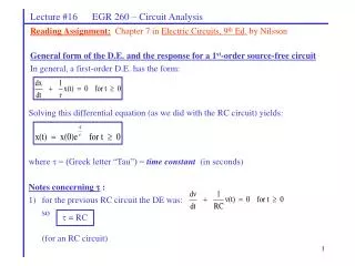
Lecture #16 EGR 260 – Circuit Analysis. Reading Assignment: Chapter 7 in Electric Circuits, 9 th Ed. by Nilsson . General form of the D.E. and the response for a 1 st -order source-free circuit In general, a first-order D.E. has the form:.

Lecture #16 EGR 260 – Circuit Analysis
E N D
Presentation Transcript
Lecture #16 EGR 260 – Circuit Analysis Reading Assignment:Chapter 7 in Electric Circuits, 9th Ed. by Nilsson General form of the D.E. and the response for a 1st-order source-free circuit In general, a first-order D.E. has the form: Solving this differential equation (as we did with the RC circuit) yields: where = (Greek letter “Tau”) = time constant (in seconds) Notes concerning : 1) for the previous RC circuit the DE was: so (for an RC circuit) = RC
Smaller t (faster decay) x(0) Larger t (slower decay) t 0 0 Lecture #16 EGR 260 – Circuit Analysis 2) is related to the rate of exponential decay in a circuit as shown below 3) It is typically easier to sketch a response in terms of multiples of than to be concerning with scaling of the graph (otherwise choosing an appropriate scale can be difficult). This is illustrated on the following page.
x(t) t 0 t 2t 3t 4t 5t Lecture #16 EGR 260 – Circuit Analysis Graphing functions in terms of : Illustration: A) Calculate values for x(t) = x(0)e-t/ for t = , 2, 3, 4, and 5. B) Graph x(t) versus t for t = 0, , 2, 3, 4, and 5.
t = tx t = tx Circuit 470uF RBleeder Lecture #16 EGR 260 – Circuit Analysis Time for a circuit to completely decay From the last page note that x(5t) = x(0)e-5t/ = x(0)e-5 = 0.007x(0) This means that magnitude of x(t) is only 0.7% of its initial value by time 5 (or the function has lost 99.3% of its original value). Technically a decaying exponential function never reaches zero, but we see that by time t = 5 it is very close. So we generally use the approximation that: 5 = time for a circuit to decay Example: Some circuits connect a “bleeder resistor” in parallel with a capacitor when the circuit is turned off in order to safely discharge the capacitor (which might otherwise have a significant voltage across it for a long time). For the circuit shown below, what value of Rbleeder should be used in order to discharge the capacitor in 10 seconds (the circuit is turned off at time t = tx)?
Lecture #16 EGR 260 – Circuit Analysis Example: The switch in the circuit shown had been closed for a long time and then opened at time t = 0. A) Determine an expression for v(t). B) Graph v(t) versus t.
Lecture #16 EGR 260 – Circuit Analysis Example: (continued) C) How long will it take for the capacitor to completely discharge? D) Determine the capacitor voltage at time t = 100 ms. E) Determine the time at which the capacitor voltage is 10V.
Circuit t > 0 independent sources killed REQ Circuit C Lecture #16 EGR 260 – Circuit Analysis Equivalent Resistance seen by a Capacitor For the RC circuit in the previous example, it was determined that = RC. But what value of R should be used in circuits with multiple resistors? In general, a first-order RC circuit has the following time constant: = REQ C where Req is the Thevenin resistance seen by the capacitor. More specifically,
Lecture #16 EGR 260 – Circuit Analysis Example: Determine an expression for v(t). Graph v(t) versus t.
Lecture #16 EGR 260 – Circuit Analysis Source-free RL circuit Consider the RL circuit shown below. Use KCL to find the differential equation: and use the general form of the solution to a first-order D.E. to show that: = L/R
Circuit t > 0 independent sources killed REQ L Circuit Lecture #16 EGR 260 – Circuit Analysis Equivalent Resistance seen by an Inductor For the RL circuit in the previous example, it was determined that = L/R. As with the RC circuit, the value of R should actually be the equivalent (or Thevenin) resistance seen by the inductor. In general, a first-order RL circuit has the following time constant: where
Lecture #16 EGR 260 – Circuit Analysis Example: Determine an expression for i(t). Sketch i(t) versus t.
Lecture #16 EGR 260 – Circuit Analysis First-order circuits with DC forcing functions: In the last class we consider source-free circuits (circuits with no independent sources for t > ). Now we will consider circuits having DC forcing functions for t > 0 (i.e., circuits that do have independent DC sources for t > 0). The general solution to a differential equation has two parts: x(t) = xh + xp = homogeneous solution + particular solution or x(t) = xn + xf = natural solution + forced solution where xh or xn is due to the initial conditions in the circuit and xp or xf is due to the forcing functions (independent voltage and current sources for t > 0). xp or xf in general take on the “form” of the forcing functions, so DC sources imply that the forced response function will be a constant (DC), Sinusoidal sources imply that the forced response will be sinusoidal, etc. Since we are only considering DC forcing functions in this chapter, we assume that xf = B (a constant)
Lecture #16 EGR 260 – Circuit Analysis Recall that a 1st-order source-free circuit had the form Ae-t/ . Note that there was a natural response only since there were no forcing functions (sources) for t > 0. So the natural response was xn = Ae-t/ The complete response for 1st-order circuit with DC forcing functions therefore will have the form x(t) = xf + xn or x(t) = B + Ae-t/ The “Shortcut Method” An easy way to find the constants B and A is to evaluate x(t) at 2 points. Two convenient points at t = 0- and t = since the circuit is in steady-state at these two points. This approach is sometimes called the “shortcut method.” So, x(0) = B + Ae0 = B + A And x() = B + Ae- = B Show how this yields the following expression found in the text: x(t) = x() +[x(0) - x()]e-t/
Lecture #16 EGR 260 – Circuit Analysis “Shortcut Method” - Procedure The shortcut method will be the key method used in this chapter to analyze 1st-order circuit with DC forcing functions: 1) Analyze the circuit at t = 0-: Find x(0-) = x(0+), where x = vC or iL . 2) Analyze the circuit at t = : Find x(). 3) Find = REQC or = L/REQ . 4) Assume that x(t) has the form x(t) = B + Ae-t/ and solve for B and A using x(0) and x(). • Notes: • The “shortcut method” also works for source-free circuits, but x() = B = 0 since the circuit is dead at t = . • If variables other than vC or iL are needed, it is generally easiest to solve for vC or iL first and then use the result to find the desired variable.
Lecture #16 EGR 260 – Circuit Analysis Example: Find v(t) and i(t) for t > 0.
Lecture #16 EGR 260 – Circuit Analysis Example: Find v(t) and i(t) for t > 0.


