f 6
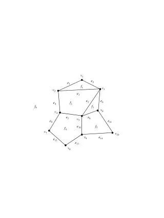
v 1. e 2. e 1. f 1. v 3. v 2. e 3. e 5. e 6. e 4. f 2. f 6. f 3. v 6. v 4. e 7. e 8. v 5. e 9. e 11. e 10. f 5. f 4. v 7. v 10. v 9. e 14. e 12. e 13. v 8. Preliminaries. Planar straight line graph A planar straight line graph (PSLG) is a planar embedding

f 6
E N D
Presentation Transcript
v1 e2 e1 f1 v3 v2 e3 e5 e6 e4 f2 f6 f3 v6 v4 e7 e8 v5 e9 e11 e10 f5 f4 v7 v10 v9 e14 e12 e13 v8
Preliminaries Planar straight line graph A planar straight line graph (PSLG) is a planar embedding of a planar graph G = (V, E) with: 1. each vertex vV mapped to a distinct point in the plane, 2. and each edge eE mapped to a segment between the points for the endpoint vertices of the edge such that no two segments intersect, except at their endpoints. edge (14) vertex (10) face (6) Observe that PSLG is defined by mapping a mathematical object (planar graph) to a geometric object (PSLG). That mapping introduces the notion of coordinates or location, which was not present in the graph (despite its planarity). We will see later that PSLGs will be useful objects. For now we focus on a data structure to represent a PSLG.
Preliminaries Doubly connected edge list (DCEL) The DCEL data structure represents a PSLG. It has one entry (“edge node” in Preparata) for each edge in the PSLG. Each entry has 6 fields: V1 Origin of the edge V2 Terminus (destination) of the edge; implies an orientation F1 Face to the left of edge, relative to V1V2 orientation F2 Face to the right of edge, relative to V1V2 orientation P1 Index of entry for first edge encountered after edge V1V2, when proceeding counterclockwise around V1 P2 Index of entry for first edge after edge V1V2, when proceeding counterclockwise around V2 v3 f4 e3 f2 e5 v2 e1 v1 e4 f1 e2 f3 v4 Example (both PSLG and DCEL are partial)
2 2 3 F2 13 8 9 4 12 F6 11 1 3 10 F3 F1 F4 6 7 6 9 5 F5 1 4 7 8 5 Edge V1 V2 LeftF RightF PredE NextE ------------------------------------------------- 1 1 2 F6 F1 7 13 2 2 3F6F2 1 4 3 34F6 F3 2 5 4 3 9 F3 F2 3 12 5 4 6F5F3 8 11 6 6 7 F5 F4 5 10 7 1 5 F5 F6 9 8 8 45 F6 F5 3 7 9 1 7 F1 F5 1 6 10 7 8 F1 F4 9 12 11 6 9 F4 F3 6 4 12 9 8 F4 F2 11 13 13 2 8 F2 F1 2 10
Preliminaries Supplementary data structures If the PSLG has N vertices, M edges and F faces then we know N - M +F = 2 by Euler’s formula. DCEL can be described by six arrays V1[1:M], V2[1:M], LeftF[1:M] Right[1:M], PredE[1:M] and NextE[1:M]. Since both the number of faces and edges are bounded by a linear function of N, we need O(N) storage for all these arrays. Define array HV[1:N] with one entry for each vertex; entry HV[i] denotes the minimum numbered edge that is incident on vertex vi and is the first row or edge index in the DCEL where vi is in V1 or V2 column. Thus for our example in the preceding slide HV=(1,1,2,3,7,5,6,10,4]. Similarly, define array HF[1:F] where F= M-N+2 ,with one entry for each face; HF[i] is the minimum numbered edge of all the edges that make the face HF[i] and is the first row or edge index in the DCEL where Fii is in LeftF or RightF column. For our example, HF=(1,2,3,6,5,1). . Both HV and HF can be filled in O(N) time each by scanning DCEL. DCEL operations Procedure EdgesIncident (“VERTEX” in Preparata) use a DCEL to report the edges incident to a vertex vj in a PSLG. The edges incident to vj are given as indexes to the DCEL entries for those edges in array A [1: 3N-6] since M<= 3N-6.
Preliminaries 1 procedure EdgesIncident(j) /* VERTEX in text */ 2 begin 3 a = HV[j] /* Get first DCEL entry for vj, a is index. */ 4 a0 = a /* Save starting index. */ 5 A[1] = a 6 i = 2 /* i is index for A */ 7 if (V1[a] = j) then /* vertex j is the origin */ 8 a =PredE[a] /* Go on to next incident edge. */ 9 else /* vertex j is the destination vertex of edge a */ 10 a =NextE[a] /* Go on to next incident edge. */ 11 endif 12 while (aa0) do /* Back to starting edge? */ 13 A[i] = a 14 if (V1[a] = j) then 15 a = PredE[a] /* Go on to next incident edge. */ 16 else 17 a = NextE[a] /* Go on to next incident edge. */ 18 endif 19 i = i + 1 20 endwhile 21 end NextE[a] V2[a] a V1[a] PredE[a]
Preliminaries DCEL notes If we make the following changes, it will become a procedure Faceincident[j] giving all the edges that constitute a face: 3: a = HF[j] And sustitute HV by HF and V1 by F1. A will have a size A[1:N]. Both EdgesIncident and Faceincident requires time proportional to the number of incident edges reported. How does that relate to N, the number of vertices in the PSLG? We have these facts about planar graphs (and thus PSLGs): (1) v - e + f = 2 Euler’s formula (2) e 3v - 6 (3) f 2/3e (4) f 2v - 4 where v = number of vertices = N e = number of edges=M f = number of faces=F vO(N) by definition eO(N) by (2) EdgesIncident requires time O(N) and DCEL requires storage O(N), one entry per edge.
(x, y) 0 a + b b a Preliminaries Vector algebra An ordered pair (x, y) can be a point in the plane, or a vector. Vector addition Given vectors a = (xa, ya) and b = (xb, yb), vector addition is defined as a + b = (xa + xb, ya + yb). Geometrically, vectors a and b determine a parallelogram with vertices 0, a, b, and a + b.
2b b 0 -b Preliminaries Scalar multiplication Multiplication of vector b by a scalar (a real number) t. Scalar multiplication is defined as tb = (txb, tyb). The vector length is scaled by t. If t < 0, the direction is reversed.
Preliminaries Vector subtraction Given vectors a = (xa, ya) and b = (xb, yb), vector subtraction is defined as b - a = b + (-1)a, carried out as b - a = (xb - xa, yb - ya). b b - a a Vector length Length of vector a = (xa, ya) is defined as |a| = sqrt(xa2 + ya2).
Vector Translation q b p a b-a o -a Let a =op and b =oq. Then, b-a is a translation of the vector pq at the origin o. Thus, two line segments having same length and direction are translates of each other and can be identified with the same canonical line segment originating at the origin o.
Preliminaries Vector direction The direction of vector a is described by its polar angle a, the angle the vector makes with the positive x axis. Measured in counterclockwise rotation, starting at the positive x axis. Values are in the range 0 a < 360. b a ab a Given two vectors a and b, the angle between them ab is measured counterclockwise starting at vector a.
Preliminaries Trigonometry reminder Definition of sine and cosine based on unit circle. 90 Unit circle x2 + y2 = 1 (x, y) 180 0 270 x = cos y = sin 0 < < 180 y > 0 sin > 0 180 < < 360 y < 0 sin < 0
p0 p1 a p2 b Preliminaries LEFT-RIGHT-ABOVE-BELOW A geometric primitive operation: triangle orientation Given three non-collinear points p0, p1, p2, the triangle p0p1p2 is positively oriented if p2 lies to the left of p0p1, and negatively oriented if p2 lies to the right of p0p1. Let vector a = p1 - p0 and vector b = p2 - p0 . p2 b ab < 180 positive orientation p0, p1, p2 form a counter-clockwise cycle + a ab p1 p0 ab < 360 negative orientation - ab p0, p1, p2 form a clockwise cycle
We introduce the value Q = b - a (note that Qab). (Equality holds if a and b are collinear.) With this information, we could compute Q = b - a and then use the table to give the orientation of p0p1p2. But computing a and b require expensive trig functions. Can we do better?
Preliminaries Observe from the table that sin(Q) has the same sign as the orientation of p0p1p2. sin(Q) = sin(b - a) by definition of Q = sin b cos a - cos b sin a by trig identity We know that cos a = xa / |a| sin a = ya / |a| cos b = xb / |b| sin b = yb / |b| by definition of sine and cosine. Then by substitution sin(b - a) = (yb / |b|)(xa / |a|) - (xb / |b|)(ya / |a|) = (1 / |a| |b|) (ybxa - xbya). |a| and |b| are positive constants, so sign(sin(b - a)) = sign(ybxa - xbya). By definition, xa = (x1 - x0) ya = (y1 - y0) xb = (x2 - x0) yb = (y2 - y0) so sign(sin(b - a)) = sign((y2 - y0)(x1 - x0) - (x2 - x0)(y1 - y0)). The latter expression can be used to find the orientation of p0p1p2 from the coordinates of p0,p1,p2 in constant time.
Preliminaries Another way of reaching the same expression is with the determinant of the coordinates of the points: | x0y0 1 | D = | x1y1 1 | | x2y2 1 | Evaluating this determinant gives the expression x0 y1 + x2 y0 + x1 y2 - x2 y1 - x0 y2 - x1 y0 which is the expansion of the final expression previously derived. Left turn/Right Turn Test If the sign of the determinant D is positive then p0p1p2 is counter- clockwise (p2 is left of p0p1 ) and if D is negative then p0p1p2 is clockwise(p2 is right of p0p1). If D=0, then the three points are collinear. p2 left p0 p1 p2 right
Area Interpretation The value of the determinant D is twice the signed area of the triangle p0p1p2 . The signed area is positive if p0p1p2 form a counter clockwise sequence, it is negative if this sequence is clockwise. If the area is zero, then D is 0. Generalizaion The three points p0 p1 and p2 form a plane in 3-d with a positive normal. A fourth point p3 is on the upside if p3 falls on the positive side of the plane and on the downside if p3 falls on the negative side of the plane. The test for this is with respect to the sig of the determinant | x0 y0 x0 1 | | x1 y1 z1 1 | D= | x2 y2 z2 1 | | x3 y3 z3 1 | This D represents the signed volume of the polyhedron. The fomulation extends to n-dimensional space. (Further Reading : Section 1:3(p.17) to Section 1:5 (p.35), in O’Rourke text).
< 0 p1 = 0 0 < < 1 p0 = 1 > 1 Preliminaries Parametric equation of a line We use the following equation of a line: line = {(p0) + (1 - (p1) }, where (real numbers) where p0 and p1 as usual are the points determining the line. p0 = (x0, y0) p1 = (x1, y1) Substituting gives {(x0, y0) + (1 - (x1, y1) } Multiplying through gives the coordinates {x0 + (1 - x1, y0 + (1 - y1 }
Note, in the previous slide,we implicitly assumedthat the points are located in a plane. The definition is valid in d- dimension where a point is specified by giving a vector of d real numbers. Thus, for three dimension, the two points can be specified as : p0=(x0,y0,z0) p1=(x1,y1,z1) And the equation for the line in parametric form will look like: line = {(p0) + (1 - (p1) }, where (real numbers) This is again the set of points in three dimension that lie on the line connecting these two points. The discussion is valid for Euclidean space Ed. If is restricted to be in the range between 0 and 1, the equation becomes the equation of the line segment connecting these two points.
Preliminaries Point-Line classification We now consider the geometric primitive operation of classifying a point w.r.t. a line (both in the plane). A directed line segment partitions the plane into 7 non-overlapping regions. The possibilities are shown below. The problem, given p0, p1, and p2, is to determine which region p2 lies in. beyond p1 left terminus between p0 origin right behind
Preliminaries Summary of geometric primitives We have seen the following primitives: 1. Triangle orientation or 2. Left/Right test 3. Point-line classification Others O(1) time operations: 1. Point-on-plane test 2. Segment-segment intersection 3. Segment-triangle intersection All require constant time (if d is fixed).