Download
1 / 58
600 likes | 1.07k Vues
Protein Structure Prediction Ram Samudrala University of Washington. Rationale for understanding protein structure and function. structure determination structure prediction. Protein structure - three dimensional - complicated - mediates function. homology rational mutagenesis

E N D
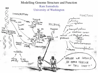
Protein Structure Prediction Ram Samudrala University of Washington
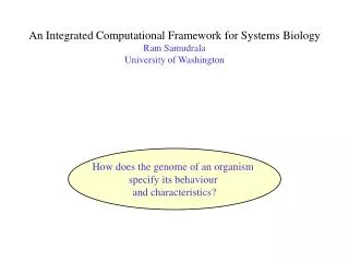
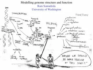
Rationale for understanding protein structure and function structure determination structure prediction Protein structure - three dimensional - complicated - mediates function homology rational mutagenesis biochemical analysis model studies Protein sequence -large numbers of sequences, including whole genomes ? Protein function - rational drug design and treatment of disease - protein and genetic engineering - build networks to model cellular pathways - study organismal function and evolution
Protein folding not unique mobile inactive expanded irregular spontaneous self-organisation (~1 second) native state DNA …-CUA-AAA-GAA-GGU-GUU-AGC-AAG-GUU-… protein sequence …-L-K-E-G-V-S-K-D-… one amino acid unfolded protein
Protein folding not unique mobile inactive expanded irregular spontaneous self-organisation (~1 second) unique shape precisely ordered stable/functional globular/compact helices and sheets native state DNA …-CUA-AAA-GAA-GGU-GUU-AGC-AAG-GUU-… protein sequence …-L-K-E-G-V-S-K-D-… one amino acid unfolded protein
Protein folding landscape Large multi-dimensional space of changing conformations J=10-3 s unfolded barrier height molten globule DG* free energy native J=10-8 s folding reaction
Protein primary structure twenty types of amino acids two amino acids join by forming a peptide bond R R H O H C H H N OH Cα Cα Cα OH N C N C H H O O H H R each residue in the amino acid main chain has two degrees of freedom (f and y) R R H O H O H H c c y f y f C N C f N f Cα Cα Cα Cα N C N C y y c c H H O H O H R R the amino acid side chains can have up to four degrees of freedom (c1-4)
Protein secondary structure many f,y combinations are not possible b sheet (anti-parallel) +180 b L a f 0 C -180 -180 0 y +180 N a helix C b sheet (parallel) N
Protein tertiary and quaternary structures Ribonuclease inhibitor (2bnh) Haemoglobin (1hbh) Hemagglutinin (1hgd)
Methods for determining protein structure X-ray crystallography NMR spectroscopy Protein structure - three dimensional - complicated - mediates function homology rational mutagenesis biochemical analysis model studies Protein sequence -large numbers of sequences, including whole genomes ? Protein function - rational drug design and treatment of disease - protein and genetic engineering - build networks to model cellular pathways - study organismal function and evolution
X-ray crystallography- concept • X-rays interact with electrons in protein molecules arranged in a crystal to produce • diffraction patterns • The diffraction patterns of the x-rays can be used to determine the three-dimensional • structure of proteins • Provides a “static” picture From <http://info.bio.cmu.edu/courses/03231/LecF01/Lec25/lec25.html>
X-ray crystallography- details • Prepare protein crystals where the proteins are organised in a precisecrystal lattice • Shine x-rays on crystals which diffract off of electrons of atoms inthe crystals; the • intensities of the individual reflections aremeasured • Phases are usually obtained indirectly by ismorphous replacement, fromthe way one or • a few heavy atoms incorporated into the sameisomorphous crystal lattice affect the • diffraction patern • Intensities and phases of all reflections are combined in a Fouriertransform to provide • maps of electron density • Interpret the map by fitting the polypeptide chain to the contours • Refine the model by minimising the distance between the observedamplitudes and the • calculated amplitudes
NMR spectroscopy - concept NK-lysin (1nkl) S1 RNA binding domain (1sro) • The magnetic-spin properties of atomic nuclei within a molecule areused to obtain a • list of distance constraints between atoms in themolecule, from which a • three-dimensional structure of the proteinmolecule can be obtained • Provides a “dynamic” picture
NMR spectroscopy - details • Protein molecules placed in a strong magnetic field have theirhydrogen atoms aligned • to the field; the alignment can be excited byapplying radio frequency (RF) pulses • Possible to obtain unique signal (chemical shift) for each hydrogenatom in a protein • molecule • Structural information arises primarily from the Nuclear OverhauserEffect (NOE), • which gives information about distances between atoms ina molecule • A pair of protons give a detectable NOE cross-peak if they are within5.0 Åof each • other in space • After obtaining NOE data for protons througout the structure, a numberof independent • structures can be generated that are consistent withthe distance constraints
Computer representation of protein structure • Structures are stored in the protein data bank (PDB), arepository of mostly • experimental models based on X-raycrystallographic and NMR studies • <http://www.rcsb.org> • Atoms are defined by their Cartesian coordinates: • ATOM 1 N GLU 1 18.222 18.496 -16.203 1.00 21.95 • ATOM 2 CA GLU 1 17.706 17.982 -14.905 1.00 16.74 • ATOM 3 C GLU 1 17.368 16.466 -15.121 1.00 15.45 • ATOM 4 O GLU 1 16.780 16.073 -16.175 1.00 18.81 • ATOM 5 CB GLU 1 16.552 18.744 -14.351 1.00 17.35 • ATOM 6 CG GLU 1 16.952 20.118 -13.803 1.00 24.48 • ATOM 7 CD GLU 1 15.881 21.145 -13.597 1.00 31.51 • ATOM 8 OE1 GLU 1 16.012 22.316 -13.292 1.00 29.12 • ATOM 9 OE2 GLU 1 14.701 20.768 -13.799 1.00 35.19 • ATOM 10 N PHE 2 17.762 15.746 -14.052 1.00 15.83 • ATOM 11 CA PHE 2 17.509 14.262 -14.184 1.00 13.24 • These structures provide the basis for most of theoretical workin protein folding and • protein structure prediction
Comparison of protein structures 3.6 Å 2.9 Å NK-lysin (1nkl) Bacteriocin T102/as48 (1e68) T102 best model • Need ways to determine if two protein structures are related and to compare predicted • models to experimental structures • Commonly used measure is the root mean square deviation (RMSD)of the Cartesian • atoms between two structures after optimalsuperposition (McLachlan, 1979): • Usually use Caatoms • Other measures include contact maps and torsion angle RMSDs
Methods for predicting protein structure comparative modelling fold recognition ab initio prediction Protein structure - three dimensional - complicated - mediates function homology rational mutagenesis biochemical analysis model studies Protein sequence -large numbers of sequences, including whole genomes ? Protein function - rational drug design and treatment of disease - protein and genetic engineering - build networks to model cellular pathways - study organismal function and evolution
Comparative modelling of protein structure • Proteins that have similar sequences (i.e., related by evolution)have similar • three-dimensional structures • A model of a protein whose structure is not known can be constructedif the structure of • a related protein has been determined byexperimental methods • Similarity must be obvious and significant for good models to be built • Need ways to build regions that are not similar between the tworelated proteins • Need ways to move model closer to the native structure
Comparative modelling of protein structure scan align KDHPFGFAVPTKNPDGTMNLMNWECAIP KDPPAGIGAPQDN----QNIMLWNAVIP ** * * * * * * * ** … … build initial model construct non-conserved side chains and main chains refine
Fold recognition 3.6 Å 5% ID NK-lysin (1nkl) Bacteriocin T102/as48 (1e68) • The number of possible protein structures/folds is limited (largenumber of sequences • but few folds) • Proteins that do not have similar sequences sometimes have similarthree-dimensional • structures • A sequence whose structure is not known is fitted directly (or“threaded”) onto a known • structure and the “goodness of fit” isevaluated using a discriminatory function • Need ways to move model closer to the native structure
Fold recognition evaluate fit KDHPFGFAVPTKNPDGTMNLMNWECAIP KDPPAGIGAPQDN----QNIMLWNAVIP ** * * * * * * * ** … … build initial model construct non-conserved side chains and main chains refine
Ab initio prediction of protein structure – concept • Go from sequence to structure by sampling the conformational space ina reasonable • manner and select a native-like conformation using a gooddiscrimination function • Problems: conformational space is astronomical, and it is hard todesign functions that • are not fooled by non-native conformations (or“decoys”)
Ab initio prediction of protein structure select sample conformational space such that native-like conformations are found hard to design functions that are not fooled by non-native conformations (“decoys”) astronomically large number of conformations 5 states/100 residues = 5100 = 1070
Sampling conformational space – continuous approaches energy • Most work in the field • Molecular dynamics • Continuous energy minimisation (follow a valley) • Monte Carlo simulation • Genetic Algorithms • Like real polypeptide folding process • Cannot be sure if native-like conformations are sampled
Molecular dynamics • Force = -dU/dx (slope of potential U); acceleration, m a(t) = force • All atoms are moving so forces between atoms are complicated functions of time • Analytical solution for x(t) and v(t) is impossible; numerical solution is trivial • Atoms move for very short times of 10-15 seconds or 0.001 picoseconds (ps) • x(t+Dt) = x(t) + v(t)Dt + [4a(t) – a(t-Dt)] Dt2/6 • v(t+Dt) = v(t) + [2a(t+Dt)+5a(t)-a(t-Dt)] Dt/6 • Ukinetic = ½ Σ mivi(t)2 = ½ n KBT • Total energy (Upotential + Ukinetic) must not change with time old position old velocity acceleration new position old velocity acceleration new velocity n is number of coordinates (not atoms)
Energy minimisation starting conformation energy deep minimum number of steps energy give up steepest descent conjugate gradient number of steps converge RMSD • For a given protein, the energy depends on thousands of x,y,z Cartesian atomic • coordinates; reaching a deep minimum is not trivial • With convergence, we have an accurate equilibrium conformation and a well-defined • energy value
Monte Carlo simulation • Discrete moves in torsion or cartesian conformational space • Evaluate energy after every move and compare to previous energy (DE) • Accept conformation based on Boltzmann probability: • Many variations, including simulated annealing (starting with ahigh temperature so • more moves are accepted initially and thencooling) • If run for infinite time, simulation will produce a Boltzmmandistribution
Genetic Algorithms • Generate an initial pool of conformations • Perform crossover and mutation operations on this set to generatea much larger pool of • conformations • Select a subset of the fittest conformations from this large pool • Repeat above two steps until convergence
Sampling conformational space – exhaustive approaches select enumerate all possible conformations view entire space (perfect partition function) must use discrete state models to minimise number of conformations explored computationally intractable: 5 states/100 residues = 5100 = 1070 possible conformations
Scoring/energy functions • Need a way to select native-like conformations from non-native ones • Physics-based functions: electrostatics, van der Waals, solvation, bond/angle terms • Knowledge-based scoring functions: derive information about atomic properties from a • database of experimentally determined conformations; common parametres include • pairwise atomic distances and amino acid burial/exposure.
Requirements for sampling methods and scoring functions • Sampling methods must produce good decoy sets that are comprehensive and include • several native-like structures • Scoring function scores must correlate well with RMSD of conformations (the better • the score/energy, the lower the RMSD)
Overview of CASP experiment • Three categories: comparative/homology modelling, foldrecognition/threading, and • ab initio prediction • Goal is to assess structure prediction methods in a blind andrigourous manner; blind • prediction is necessary for accurateassessment of methods • Ask modellers to build models of structures as they are in the processof being solved • experimentally • After prediction season is over, compare predicted models to theexperimental • structures • Discuss what went right, what went wrong, and why • Compare progress from CASP1 to CASP4 • Results published in special issues of Proteins: Structure, Function, Genetics 1995, • 1997, 1999, 2002
Comparative modelling at CASP - methods • Alignment: PSI-BLAST, FASTA, CLUSTALW - multiple sequencealignments • carefully hand-edited using secondary structure information • More successful side chain prediction methods include: • backbone-dependent rotamer libraries (Bower & Dunbrack) • segment matching followed by energy minimisation (Levitt) • self-consistent mean field optimisation (Bates et al) • graph-theory+ knowledge-basedfunctions (Samudrala et al) • More successful loop building methods include: • satisfaction of spatial restraints (Sali) • internal coordinate mechanics energy optimisation (Abagyan et al) • graph-theory + knowledge-basedfunctions (Samudrala et al) • Overall model building: there is no substitute for careful hand-constructed models • (Sternberg et al, Venclovas)
A graph theoretic representation of protein structure -0.6 (V1) represent residues as nodes -0.5 (I) -0.9 (V2) weigh nodes -0.7 (K) -1.0 (F) construct graph -0.6 (V1) -0.2 -0.5 (I) -0.9 (V2) -0.1 -0.5 (I) -0.9 (V2) -0.1 -0.1 -0.3 -0.1 find cliques -0.2 -0.4 -0.3 -0.1 -0.1 -0.4 W = -4.5 -0.2 -0.7 (K) -1.0 (F) -0.2 -0.7 (K) -1.0 (F)
Historical perspective on comparative modelling alignment side chain short loops longer loops BC excellent ~ 80% 1.0 Å 2.0 Å
Historical perspective on comparative modelling alignment side chain short loops longer loops BC excellent ~ 80% 1.0 Å 2.0 Å CASP1 poor ~ 50% ~ 3.0 Å > 5.0 Å
Prediction for CASP4 target T128/sodm Ca RMSD of 1.0 Å for 198 residues (PID 50%)
Prediction for CASP4 target T111/eno Ca RMSD of 1.7 Å for 430 residues (PID 51%)
Prediction for CASP4 target T122/trpa Ca RMSD of 2.9 Å for 241 residues (PID 33%)
Prediction for CASP4 target T125/sp18 Ca RMSD of 4.4 Å for 137 residues (PID 24%)
Prediction for CASP4 target T112/dhso Ca RMSD of 4.9 Å for 348 residues (PID 24%)
Prediction for CASP4 target T92/yeco Ca RMSD of 5.6 Å for 104 residues (PID 12%)
Comparative modelling at CASP - conclusions alignment side chain short loops longer loops BC excellent ~ 80% 1.0 Å 2.0 Å CASP1 poor ~ 50% ~ 3.0 Å > 5.0 Å CASP2 fair ~ 75% ~ 1.0 Å ~ 3.0 Å CASP3 fair ~75% ~ 1.0 Å ~ 2.5 Å CASP4 fair ~75% ~ 1.0 Å ~ 2.0 Å CASP4: overall model accuracy ranging from 1 Å to 6 Å for 50-10% sequence identity **T111/eno – 1.7 Å (430 residues; 51%) **T122/trpa – 2.9 Å (241 residues; 33%) **T128/sodm – 1.0 Å (198 residues; 50%) **T125/sp18 – 4.4 Å (137 residues; 24%) **T112/dhso – 4.9 Å (348 residues; 24%) **T92/yeco – 5.6 Å (104 residues; 12%)
Fold recognition at CASP - methods • Visual inspection with sequence comparison (Murzin group) • Procyon - potential of mean force based on pairwise interactionsand global dynamic • programming (Sippl group) • Threader - potential of mean force and double dynamic programming (Jones group) • Environmental 3D Profiles (Eisenberg group) • NCBI Threading Program using contact potentials and models ofsequence-structure • conservation (Bryant group) • Hidden Markov Models (Karplus group) • Combination of threading with ab initio approaches (Friesner group) • Environment-specific substitution tables and structure-dependent gap penalties • (Blundell group)
Fold recognition at CASP - conclusions • Fold recognition is one of the more successful approaches atpredicting structure at all • four CASPs • At CASP2 and CASP4, one of the best methods was simple sequence searching with • carefulmanual inspection (Murzin group) • At CASP3 and CASP4, none of the threading targets could have been recognised bythe • best standard sequence comparison methods such asPSI-BLAST • For the most difficult targets, the methods were able to predict 60 residuesto 6.0Å • Ca RMSD, approaching comparative modelling accuracies as the similarity between • proteins increased.
Ab initio prediction at CASP – methods • Assembly of fragments with simulated annealing (Simons et al) • Exhaustive sampling and pruning using knowledge-based scoringfunctions • (Samudrala et al) • Constraint-based Monte Carlo optimisation (Skolnick et al) • Thermodynamic model for secondary structure prediction withmanual docking of • secondary structure elements and minimisation(Lomize et al) • Minimisation of a physical potential energy function with asimplified representation • (Scheraga et al, Osguthorpe et al) • Neural networks to predict secondary structure (Jones, Rost)
Semi-exhaustive segment-based folding fragments from database 14-state f,y model generate … … monte carlo with simulated annealing conformational space annealing, GA minimise … … all-atom pairwise interactions, bad contacts compactness, secondary structure filter EFDVILKAAGANKVAVIKAVRGATGLGLKEAKDLVESAPAALKEGVSKDDAEALKKALEEAGAEVEVK
Historical perspective on ab initio prediction Before CASP (BC): “solved” (biased results) CASP2: worse than random with one exception CASP1: worse than random CASP3: consistently predicted correct topology - ~ 6.0 Å for 60+ residues *T56/dnab – 6.8 Å (60 residues; 67-126) **T61/hdea – 7.4 Å (66 residues; 9-74) **T64/sinr – 4.8 Å (68 residues; 1-68) **T75/ets1 – 7.7 Å (77 residues; 55-131) *T74/eps15 – 7.0 Å (60 residues; 154-213) **T59/smd3 – 6.8 Å (46 residues; 30-75) CASP4: ?
Prediction for CASP4 target T110/rbfa Ca RMSD of 4.0 Å for 80 residues (1-80)
Prediction for CASP4 target T97/er29 Ca RMSD of 6.2 Å for 80 residues (18-97)
Prediction for CASP4 target T106/sfrp3 Ca RMSD of 6.2 Å for 70 residues (6-75)