Download
1 / 39
420 likes | 664 Vues
Two Species Model of Epidemic Spreading. Ahn, Yong-Yeol. 2005.4.14. Epidemics and Contact Process. Epidemics is about self-replicators which can die . Contact process : A simple model consists of branching and spontaneous annihilation. Contact Process. λ. λ = ν / δ. 1. v.

E N D
Two Species Model of Epidemic Spreading Ahn, Yong-Yeol. 2005.4.14
Epidemics and Contact Process • Epidemics is about self-replicators which can die. • Contact process : A simple model consists of branching and spontaneous annihilation.
Contact Process λ λ=ν/ δ 1 v
Contact Process We can NOT solve exactly this terribly simple process! Approx. Malthus–Verhulst eq. For λ < 0 infection vanishes. For λ > 0 steady state ( i = 1 – 1/ λ) This equation is “wrong”, but correctly describes the qualitative dynamics of contact process, which is that… Contact process exhibits an absorbing phase transition.
Absorbing Phase Transition • Order parameter • Correlation length • Correlation time ρ inactive active p
Directed Percolation • Contact process is same as the directed percolation process. • In the lattice with randomly occupied edges, • Follow only occupied edges in only designated direction. • This process can continue ad infinitum? Directed Percolation problem
Surface Roughening Model and DP - Let’s see only one layer No spontaneous infection no digging condition X
S. R. and Coupled DP (RSOS : Restricted solid-on-solid interface) A A A A A B B B B B B B B B B C C C C C C C C C C C C D D D D D D D D D D D D D active inactive
Asymmetrically Coupled DP Positive coupling A B C D .. Negative coupling • Simulation results in 1D • A : DP critical behavior • B, C, … : dressed • negative coupling is irrelevant
A B ACDP : Diagram Detection and initiation Antibody Worm killing worm Antigen Contagion Healing
ACDP on Networks • Antigen – antibody interaction • Worm – worm killing worm • Motto: “Never flood the network”
Phase Diagram • If there is no virus, vaccine spreading has a epidemic threshold. • If there is no vaccine, virus has no epidemic threshold. Vaccine Annihilation probability There is the happy region where there is no virus and no vaccine. Virus Annihilation probability
Mean Field Theory Mean field eq. At ‘M’ DP DP DP
On a Scale-Free Network • We should consider each degree seperately.
SIS Model on a Scale-free Network Because a scale-free network is very inhomogenous, we must consider the density of infected nodes seperately for each degree. is the probability that any given link points to an infected node. (We don’t need to consider the excess degree because we’re dealing with SIS model. )
SIS Model on a Scale-free Network The probability that the selected node is not infected
SIS Model on a Scale-free Network ρk = ik At Steady state, Edge selection Average degree Where With these two equations and continum approximation, We get
SIS Model on a Scale-free Network • By solving previous equation, we get, “no epidemic threshold on the scale-free network” Scale-free Vanishing Epidemic threshold Homogeneous network
infecting or activating vaccine at “all neighbors” with prob. spontaneous annihilation with prob. predation spontaneous annihilation with prob. branching“one offspring” with prob. CDP on a Scale-free Network From J.D. Noh’s ppt
Different Branching Rule • Because we do not want the vaccine occupying the whole network and vaccine is more active in the condition that virus is abundant, we assign a different rule for the vaccine. • Both rules are possible in our CDP framework Modified rule Previous SIS rule
On a Scale-Free Network Mean field equation
When There is no Virus Mean field eq. Without degree-degree correlation,
Mean Field eq. By assuming a steady state, multiplying p(k), and summing over k, we get a equation Note that the critical point pB=½.
MF eq. And by direct calculation, • Calculating with 2<γ<3, As γ decreases, β increases. pc
MF eq. • Calculating with γ=3 β = 1 with logarithmic correction • Calculating with γ>3, β = 1 β = 1 w/ log. correction β = 1/(γ-2) β = 1 γ 3 2
Diffusion – Annihilation Process Out CDP eq. by multiflying P(k) and summing over k, When ,
Diffusion – Annihilation Process Meanwhile, diffusion-annihilation process can be described as, Same eq. And by summing over P(k),
γ 3 2 DA Process and Time Evolution • At critical point, DA process and our model is described by the same mf eq. And we apply the DA result to our model.
Simulation Result γ =3 Critical point = 0.425 (mean field : 0.5) δ = 1.3 (mf: 1 with log. correction ) δ=1.3 If we draw with logarithmic term, δ ~ 1.1
Finite Size Scaling Assuming a scaling form, ( θ=β/ν )
β =1.3 Finite Size Scaling γ =3 θ~β/ν Mf: β = 1 with log. correction
Another γs • γ =2.5 Critical point = 0.425 (mean field : 0.5) δ = 2.0 (mf: 1/(γ-2) = 2 )
Another γs • γ =2.5 β = 1.75 (mf: 2)
Another γs • γ =2.75, 4 pc = 0.425 pc = 0.426 δ ~ 1.5 δ ~ 1.3
Summary : δ ~1.3 (1.1 w l.c.) (mf:1 w lc) 2.5 2.75 4 γ 3 2 ~1.3 (mf: 2) 2 (mf: 2) ~1.5 (mf:1.33)
β = 1 w/ log. correction β = 1/(γ-2) β = 1 γ 3 2 Summary : β ~1.3 2.75 2.5 4 Not yet Not yet 1.75 (mf:2)
Summary • We put the CDP model on a scale-free network for simulating the behavior of an epidemic and reacting anti-pathogen. • The simulation results are consistent to the mean field calculation.
References • U. C. Täuber et al., Phys. Rev. Lett. 80, 2165 (1998); Y. Y. Goldschmidt, ibid. 81, 2178 (1998). • J. D. Noh and H. Park, CondMat/051542 (to be published in Phys. Rev. Lett.). • J. Marro and R. Dickman, “Nonequilibrium Phase Transition in Lattice Models”. • Papers in http://janice.kaist.ac.kr/bbs/viewtopic.php?t=30 and related papers. • Haye Hinrichsen, “Nonequilibrium Critical Phenomena and Phase Transitions into Absorbing States”, arXiv:cond-mat/0001070. • Arno Karlen, “Man and Microbes”. • J. D. Murray, “Mathematical Biology”. • M. E. J. Newman, SIAM Review, 45, 167 (2003). • Malcolm Gladwell, “The Tipping Point”. • About percolation : 손승우, http://stat.kaist.ac.kr/~sonswoo/prl.html .