Download
1 / 37
370 likes | 511 Vues
Intermingling of two Pseudocalanus species on Georges Bank. D.J. McGillicuddy, Jr. Woods Hole Oceanographic Institution A. Bucklin University of New Hampshire Journal of Marine Research 60 , pp. 583-604, 2002. 1997 Broadscale Survey Data. P. moultoni. P. newmani. Species-specific PCR

E N D
Intermingling of two Pseudocalanusspecies on Georges Bank D.J. McGillicuddy, Jr. Woods Hole Oceanographic Institution A. Bucklin University of New Hampshire Journal of Marine Research 60, pp. 583-604, 2002.
1997 Broadscale Survey Data P. moultoni P. newmani Species-specific PCR (Bucklin et al., 2001)
The forward model: an advection-diffusion-reaction equation Tendency Diffusion Reaction (biological sources and sinks) Advection C concentration v velocity K diffusivity Cobs(t0) Cobs(t1) time The forward problem
Observations: P. Moultoni Models Observations: P. newmani
Are the inverse solutions ecologically realistic? R(x,y,t) bounded by –100 to +100 individuals m-3 day-1 [most fall between -10 to +10] C5 moulting potential: Mean C5 abundance 2500 individuals m-3 (Incze pump samples: April 1997, May 1997, June 1995) Stage duration in GB conditions: 5 days (McLaren et al., 1989) Implied moulting flux of 500 individuals m-3 day-1
Are the inverse solutions ecologically realistic? Predation potential: Model predicted rates of 3-10% day-1 Bollens et al. specific rates of predation on C. finmarchicus and Pseudocalanus spp. copepodites based on observed predator abundance and feeding rates http://userwww.sfsu.edu/~bioocean/research/gbpredation/gbpredation1.html
Conclusions (I) • Inverse method results in convergent solutions • Geographically specific regions of growth/mortality • These vary seasonally according to animal abundance • patterns, the circulation, and their orientation • Two main balances: • Tendency / source (weak currents or aligned gradients) • Tendency / source / advection
Conclusions (II) Resulting biological sources and sinks ecologically realistic -- R(x,y,t) bounded by independent rate estimates C5 moulting flux Predation by invertebrates and vertebrates Emerging conceptual model: -- Distinct source regions in late winter P. moultoni on NW flank P. newmani on NE peak and Browns Bank -- During the growing season, GB circulation blends these reproducing (not interbreeding) populations such that their distributions overlap by early summer.
Caveats Physics -- errors in the circulation -- vertical shear Biology -- density dependence vs. “geographic” formulation -- multistage models, behavior, etc. Observational limitations -- only adults -- upper 40m
Are the inverse solutions ecologically realistic? R(x,y,t) bounded by –100 to +100 individuals m-3 day-1 [most fall between -10 to +10] C5 moulting potential: Mean C5 abundance 2500 individuals m-3 (Incze pump samples) Stage duration in GB conditions: 5 days (McLaren et al., 1989) Implied moulting flux of 500 individuals m-3 day-1 Predation potential: Hydroid ingestion rate: 0.25 cop. hydr-1 day-1 (Madin et al., 1996) Characteristic abundance: 10,000 hydranths m-3 Potential consumption rate: 2500 copepods m-3 day-1 Pseudocalanus adults ~15% of total postlarvae (Davis, 1987) Hydroid predation on Pseudocalanus: 200 individuals m-3 day-1
Pseudocalanus spp.MARMAP 1977-1987 Two population centers: Western Gulf of Maine Georges Bank Davis (1984) hypothesis: Western Gulf of Maine is a source region for the Georges Bank population Concentration (# m-3)
General circulation during the stratified season Beardsley et al. (1997)
Derivation of the adjoint model (1) Define a cost function J: Problem: Given observations C0(t0) and C1(t1), find R(x,y) that minimizes J Where λ=λ(x,y,t) are Lagrange multipliers
Derivation of the adjoint model (2) We require R at the minimum of (and therefore J) where Adjoint model: It can be shown that:
Example results: Mar-Apr to May-Jun Red: source Blue: sink
Term-by-Term Diagnosis Observations Biological Source/Sink Advection Diffusion Tendency JF-MA MA-MJ MJ-JA
Chlorophyll-aMARMAP 1977-1987O’Reilly and Zetlin (1996) Jan-Feb Mar-Apr May-Jun Jul-Aug Davis (1984) Cutoff for food limitation 0.6 – 1.2 μg Chl l-1 Nov-Dec Sep-Oct Cutoff range
ChaetognathsMARMAP 1977-1987Sullivan and Meise (1996) Jan-Feb Mar-Apr May-Jun Jul-Aug Sep-Oct Nov-Dec
ECOHAB-GOM Observations • Gulf-wide • distribution • 2) Association with coastal • current • 3) Center of mass • shifts west-to-east • as season progresses Townsend et al. (2001)
Some thoughts on model designfor HAB applications Forward models Inverse approaches McG et al. (1998) Fisheries Oceanography, 7(3/4), 205-218. McG and Bucklin (2002) Journal of Marine Research, 60, 583-604. http://science.whoi.edu/users/mcgillic/software/scotia_1.0/
Term-by-Term Diagnosis Continued… Observations Biological Source/Sink Advection Diffusion Tendency JA-SO SO-ND ND-JF
Pseudocalanus spp.MARMAP 1977-1987 Concentration (# m-3)
Term-by-Term Diagnosis Obs Src Adv Dif Ten JF-MA MA-MJ MJ-JA JA-SO SO-ND ND-JF
Term-by-Term Diagnosis Obs Src Adv Dif Ten JF-MA MA-MJ MJ-JA JA-SO SO-ND ND-JF
Term-by-term diagnosis Red: source Blue: sink
Observations: P. Moultoni Models Observations: P. newmani