Chapter 12: INCOMPRESSIBLE FLOW
Chapter 12: INCOMPRESSIBLE FLOW. Effect Of Area Change. One-Dimensional Compressible Flow. R x. P 2. P 1. dQ/dt. Surface force from friction and pressure. heat/cool. (+ s 1 , h 1 ). (+ s 2 , h 2 ). What can affect fluid properties?

Chapter 12: INCOMPRESSIBLE FLOW
E N D
Presentation Transcript
Chapter 12: INCOMPRESSIBLE FLOW Effect Of Area Change
One-Dimensional Compressible Flow Rx P2 P1 dQ/dt Surface force from friction and pressure heat/cool (+ s1, h1) (+ s2, h2) What can affect fluid properties? Changing area, heating, cooling, friction, normal shock
Only change in area No heat transfer No shock No friction isentropic
Rx = pressure force along walls, no friction Rx A + dA (= 1V1A1 = 2V2A2 ) A 1-D, steady, isentropic flow with area change; no friction, no heat exchange or change in potential energy or entropy
No Friction 0 adiabatic = ho s2 = s1= const 0 C A L O R I C A L L Y I D E A L G A S CONSTANT 0 Isentropic so Q = 0, Rx is only pressure forces – no friction
Q = 0 S = constant S = constant
h = cp T, so processes plotted on Ts diagram will look similar on hs diagram
* Total energy* of flowing fluid: h + ½ V2 = constant = ho
For isentropic flow if the fluid accelerates what happens to the temperature?
For isentropic flow if the fluid accelerates what happens to the temperature? if V2>V1 then h2<h1
For isentropic flow if the fluid accelerates what happens to the temperature? if V2>V1 then h2<h1 if h2<h1 then T2<T1 Temperature Decreases
Isentropic so: s = const = so and h + V2/2 = const = ho Follows that stagnation properties are constant for all states in an isentropic flow.
If ho and so constant then po To and o are constant since anyone thermodynamic variable can be expressed as a function of any two other.
Seven nonlinear coupled equations, if isentropic and know for example: A1, p1,T1, h1,u1, 1 and A2 then could solve for p2, T2, h2, u2, 2, s2 and Rx
Hard to solve (nonlinear & coupled) so will develop property relations in terms of local stagnation conditions and critical conditions. But first lets look at general relationships e.g. how does V & p change with area
Question? As dA varies, what happens to dV and dp?
Differential form of momentum equation for steady, inviscid, quasi- one-dimensional flow (Euler’s Equation) from section 11-3.1 ~ FSx = cs VxV dA no body forces, frictionless, steady FSx = (p + dp/2)dA + pA – (p+dp)(A + dA) cs VxV dA = Vx{-VxA} + (Vx + d Vx)[( + d )(Vx + d Vx)(A + dA) dp/ + d{Vx2/2} = 0
Differential form of momentum equation for steady, inviscid, quasi- one-dimensional flow (Euler’s Equation) FSx = (p + dp/2)dA + pA – (p+dp)(A + dA) cs VxV dA = Vx{-VxA} + (Vx + d Vx)[( + d )(Vx + d Vx)(A + dA) pdA + (dp/2)dA + pA – pA – pdA – dpA – dpdA = -VxVxA + (Vx + d Vx)[VxVxA] -Adp =dVxVxVxA dp/ + d{Vx2/2} = 0 ~ 0 ~ 0
dp/ + d{Vx2/2} = 0* NOTE: Changes in pressure and velocity always have opposite sign *True along streamline in steady, inviscid flow (no body forces)
Rx = pressure force along walls, no friction p + ½ dp/dx Rx ½ dA {p + ½ dp/dx}dA = Fx 1-D, steady, isentropic flow with area change; no friction, no heat exchange or change in potential energy or entropy
EQ. 11.19b EQ.12.1a {d(AV) + dA(V) +dV(A)}/{AV} = 0 steady isentropic, steady
EQ. 12.5 EQ.12.6 isentropic, steady
Although cannot use these equations for computation since don’t know how M varies with A, still can provide interesting insight into how pressure and velocity change with area.
isentropic, steady, ~1-D Subsonic Nozzle Subsonic Diffuser M<1 If M < 1 then [ 1 – M2] is +, then dA and dP are same sign; and dA and dV are opposite sign qualitatively like incompressible flow
isentropic, steady, ~1-D Supersonic Nozzle Supersonic Diffuser M>1 If M > 1 then [ 1 – M2] is -, then dA and dP are opposite sign; and dA and dV are the same sign qualitatively not like incompressible flow
Note on counterintuitive supersonic results: Both dV and dA can be same sign because d can be opposite sign
Note on counterintuitive supersonic results: e.g. in a supersonic nozzle both dV and dA can be same sign because d is the opposite sign and large.
Flow is continuously accelerating, dV is always positive So when M<1, dA must be negative so –dA is positive So when M>1, dA must be positive so –dA is negative
Flow is continuously decelerating, dV is always negative So when M>1, dA must be negative so -dA is positive So when M<1, dA must be positive so –dA is negative
Same shape, but in one case accelerating flow, and in the other decelerating flow
isentropic, steady ~ 1-D If M = 1 then I have a problem, Eqs. 12.5 and 12.6 blow up! Only if dA 0 as M 1 can avoid singularity. Hence for isentropic flows sonic conditions can only occur where the area is constant!!!
isentropic, steady ~ 1-D Note: if incompressible, c = & M = 0 and Eq 12.6 becomes: AdV + VdA = 0 dV and dA have opposite signs or d(AV) = 0 or AV = constant (continuity equation for incompressible flow).
Same shape, but in one case accelerating flow, and in the other decelerating flow dA = constant
Computations are tedious, but because s = 0 use reference stagnation and critical conditions po/p = [1 + (k-1)M2/2]k/(k-1) To/T = 1 + (k-1)M2/2 o/ = [1 + (k-1)M2/2]1/(k-1) Strategy: if know M1 & p1, can calculate p01; But p01 = p02, so if know M2 can calculate p2. Need to know how M changes with A
Need two reference states because the reference stagnation State does not provide area information (mathematically the stagnation area is infinite.)
A S I D E Why is T* (critical temperature) less than To (stagnation temperature)?
Why is T* (critical temperature) less than To (stagnation temperature)? A S I D E Isentropic so ~ h0 = h* + V*2/2 ho = cpTo and h* = cpT* (ideal and constant cp) cpTo = cpT*+ c2/2 To = T* + c2/(2cp)
A S I D E (11.20) To /T = 1 + M2(k-1)/2 so To = T* (1 +(k-1)/2) k = 1.4 for ideal gas so To > T*
Back to problem, want to come up with easier way of manipulating these equations. Strategy: use isentropic reference conditions
EQ. 11.19b + EQ. 11.12c p / k = constant Eqs. 11.20a,b,c = Eqs. 12.7a,b,c (po, To refer to stagnation properties) isentropic, steady, ideal gas
If M = 1 the critical state; p*, T*, *…. Critical conditions related to stagnation Local conditions related to stagnation EQ. 11.17 c = [kRT]1/2 c* = [kRT*]1/2 isentropic, steady, ideal gas
Can use stagnation conditions to go from 1, p1, T1, c1 to 2, p2, T2, c2; but not A. Missing relation for area since stagnation state does not provide area information. So to get area information use critical conditions as reference.
EQ. 12.7c EQ. 11.21b EQ. 12.7b EQ. 11.21c
AxAy = Ax+y 1/(k-1) + ½ = 2/2(k-1) +(k-1)/2(k-1) = (k+1)/(2(k-1)
EQs. 12.7a,b,c,d Provide property relations in terms of local Mach numbers, critical conditions, and stagnation conditions. NOT COUPLED LIKE Eqs. 12.2, so easier to use. isentropic, ideal gas, steady, only body forces
In practice this is not shape of wind tunnel. To reduce chance of separation, divergence angle must be less severe. accelerating
For accelerating flows, favorable pressure gradient, • the idealization of isentropic flow is generally a • realistic model of the actual flow behavior. • For decelerating flows (unfavorable pressure • gradient) real fluid tend to exhibit nonisentropic • behavior such as boundary layer separation, and • formation of shock waves. accelerating