Download
1 / 138
1.55k likes | 2.47k Vues
Chapter 8: Internal Incompressible Viscous Flow. Chapter 8: Internal Incompressible Viscous Flow. Flows: Laminar (some have analytic solutions) Turbulent ( no analytic solutions) Depends of Reynolds number, Re = Inertial Force/Viscous Force. Re = L u/

E N D
Chapter 8: Internal Incompressible Viscous Flow
Chapter 8: Internal Incompressible Viscous Flow Flows: Laminar (some have analytic solutions) Turbulent (no analytic solutions) Depends of Reynolds number, Re = Inertial Force/Viscous Force
Re = Lu/ cartoon approach
REYNOLDS NUMBER = I.F./V.F. (cartoon approach) Reynolds Number ~ ratio of inertial to viscous for (Cartoon approach)ces -- hand waving argument -- Inertial Force = (m) x (a)(l3)x (U/t) U/t U/(L/U) U2/L Inertial Force (l3 )x(U2/L) Inertial Force ( L3 )x(U2/L) = L2U2 L fluid element U f
REYNOLDS NUMBER = I.F./V.F. (cartoon approach) Reynolds Number ~ ratio of inertial to viscous for (Cartoon approach)ces -- hand waving argument -- Viscous Force = () x (Area)(dU/dy) xl2 dU/dy U/l ViscousForce (U/l) xl2 ul Ul L fluid element U f
REYNOLDS NUMBER = I.F./V.F. (cartoon approach) Reynolds Number ~ ratio of inertial to viscous for (Cartoon approach)ces -- hand waving argument -- Inertial Force L2U2 ViscousForce UL L Define Re as LU/ where L & U are some characteristic length scales
Re = Lu/ from N. S. E.
REYNOLDS NUMBER a la N.S.E. a = Du/Dt = F Eq. 5.27a: (u/t + uu/x + vu/y + wu/z) = - p/x + (2u/x2 + 2u/y2 + 2u/z2) x-component incompressible, constant , Newtonian, ignore gravity, e-m, … forces,
REYNOLDS NUMBER a la N.S.E. (u/t + uu/x + vu/y + wu/z) = - p/x + (2u/x2 + 2u/y2 + 2u/z2) Let u’ = u/U, v’ = v/U, w’ = w/U; x’ = x/L, y’ = y/L, z’ = z/L; t’ = t/T and p’ = p/ (U2) L and U are characteristic lengths and velocities and T=L/U (Uu’)/(Tt’) + Uu’(Uu’)/(Lx’) + Uv’(Uu’)/(Ly’) + Uw’(Uu’)/(Lz’) = - (1/) p’U2 /Lx’ + (2(Uu’)/(Lx’)2 + 2(Uu’)/(Ly’)2 + 2(Uu’/(Lz’)2
REYNOLDS NUMBER a la N.S.E. (Uu’)/(Tt’) + Uu’(Uu’)/(Lx’) + Uv’(Uu’)/(Ly’) + Uw’(Uu’)/(Lz’) = - (1/) p’U2 /Lx’ + (2(Uu’)/(Lx’)2 + 2(Uu’)/(Ly’)2 + 2(Uu’/(Lz’)2 U/T = U/(L/U) = U2/L {U2/L}[u’/t’+u’u’/x’+v’u’/y’+w’u’/z’] = - {U2/L}p’/x’ + {U/L2}(2u’/x’2 + 2u’/y’2 + 2u’/z’2)
REYNOLDS NUMBER a la N.S.E. {U2/L}[u’/t’+u’u’/x’+v’u’/y’+w’u’/z’] = - {U2/L}p’/x’ + {U/L2}(2u’/x’2 + 2u’/y’2 + 2u’/z’2) [u’/t’ + u’u’/x’ + v’u’/y’ + w’u’/z’] = - p’/x’ + {1/[UL]}(2u’/x’2 + 2u’/y’2 + 2u’/z’2) 1/ReL
REYNOLDS NUMBER a la N.S.E. [u’/t’ + u’u’/x’ + v’u’/y’ + w’u’/z’] = - p’/x’ + {1/ReL}(2u’/x’2 + 2u’/y’2 + 2u’/z’2) High Re # in some ways independent of viscosity. However, near wall viscosity always important! (why?)
REYNOLDS NUMBER a la N.S.E. [u’/t’ + u’u’/x’ + v’u’/y’ + w’u’/z’] = - p’/x’ + {1/ReL}(2u’/x’2 + 2u’/y’2 + 2u’/z’2) High Re # in some ways independent of viscosity. However, near wall viscosity always important! (because velocity gradients large)
REYNOLDS NUMBER a la N.S.E. [u’/t’ + u’u’/x’ + v’u’/y’ + w’u’/z’] = - p’/x’ + {1/ReL}(2u’/x’2 + 2u’/y’2 + 2u’/z’2) Two flows with the same geometry, same ReL and satisfying the above equation (i.e. no body forces, incompressible, constant visosity, Newtonian) will have similar flow fields (dynamic similarity). Hence drag forces measured in the lab can be extrapolated to full scale!
The principle of dynamic similarity makes it possible to predict the performance of full-scale aircraft from wind tunnel tests. Drag coefficient is same for dynamically similar flows Drag coefficient = Drag Force / (U2L2) Lift coefficient = Lift Force / (U2L2)
REYNOLDS NUMBER - EMPIRACLE Reynolds conducted many experiments using glass tubes of 7,9, 15 and 27 mm diameter and water temperatures from 4o to 44oC. He discovered that transition from laminar to turbulent flow occurred for a critical value of uD/ (or uD/), regardless of individual values of or u or D or . ~ Nakayama & Boucher Sommerfeld in a 1908 paper first referred to uD/ as the Reynolds number
REYNOLDS NUMBER - EMPIRACLE Reynolds found that the quality of the pipe inlet affected transition – with a smoother, bell-mouthed inlet transition was delayed to higher Reynolds numbers. Laminar pipe flow is stable to infinitesimal disturbances. From Reynolds’ 1883 paper
Reynolds found transition to occur around Re = 13,000, when experiment repeated a hundred years later (left) transition was found to be much less – WHY?
Note: In pipe flow turbulence does not suddenly at Retr appear throughout the pipe. It forms turbulent slugs near the pipe entrance and grows as it is passed through the pipe.
Pipe centerline: (a) fluctuating velocity; (b) mean velocity u fluctuation u mean ----- from Triton Re = 2550
QUESTION: refer to data above, head not changing, roughness not changing, viscosity not changing, pipe diameter not changing – so why is flow rate?
Flow rate is reduced with appearance of turbulent “slug”. Flow slows down cause increased wall friction due to turbulence. If near Recr then new Re can be < Recr so no turbulent slugs near entrance. After turbulent slug passes, flow speeds up and Recr reoccurs and pattern repeats.
Chapter 8: Internal Incompressible Viscous Flow “viscous forces are dominant” - MYO Internal Flows can be: developing flows - velocity profile changing fully developed - velocity profile not changing
Chapter 8: Internal Incompressible Viscous Flow V=0 AT WALL D = 27 mm Vavg = 6 cm/sec ReD = 1600 V=0 AT WALL Internal Flows can be: developing flows - velocity profile changing fully developed - velocity profile not changing
As “inviscid” core accelerates, pressure must drop Laminar Pipe Flow Entrance Length for Fully Developed Flow L/D = 0.06 Re {L/D = 0.03 Re, Smits} {L/D = 0.06 Re, White} {L/D = 0.13 Re, Boussinesq 1891} ? Pressure gradient balances wall shear stress No acceleration
As “inviscid” core accelerates, pressure must drop Pressure gradient balances both wall shear stress and acceleration Pressure gradient balances wall shear stress No acceleration Le = 140D, Re = 2300 {same trends for turbulent flow}
As “inviscid” core accelerates, pressure must drop Turbulent Pipe Flow Entrance Length for Fully Developed Flow 25-40 pipe diameter - Fox… Le/D = 4.4 Re1/6 - MYO 20D < Le < 30D 104 < Re < 105 = White Pressure gradient balances wall shear stress No average acceleration Entrance length much shorter now in turbulent flow
LAMINAR Pipe Flow Re< 2300 (2100 for MYO) PIPE ReD = 1600 LAMINAR Duct Flow Re<1500 (2000 for SMITS) DUCT FLOW: H = 0.2 cm, Uavg = 3.2 cm, ReH = 64
Fully Developed Laminar Pipe/Duct Flow LAMINAR Pipe Flow Re< 2300 (2100 for MYO) LAMINAR Duct Flow Re<1500 (2000 for SMITS) Uo= V = Q/A OUTSIDE BLUNDARY LAYER TREAT AS INVISCID, CAN USE B.E.
Chapter 8: Internal Incompressible Viscous Flow • Compressibility requires work, may produce heat and • change temperature (note temperature changes due • to viscous dissipation usually not important) • For water usually considered constant • For gas usually considered constant for M < 0.3 • (~100m/s or 230 mph; / ~ 4%) • Pressure drop in pipes “usually” not large enough to • make compressibility an issue (water hammer in an • exception).
Time Out Static / Dynamic / Stagnation Pressures
What are static, dynamic and stagnation pressures? The thermodynamic pressure, p, used throughout this book refers to the static pressure. This is the pressure experienced by a fluid particle as it moves with the fluid. staticpressure
What are static, stagnation, and dynamic pressures? The stagnation pressure is obtained when the fluid is decelerated to zero speed through an isentropic process (no heat transfer, no friction). For incompressible flow: po = p + ½ V2
What are static, dynamic and stagnation pressures? The dynamic pressure is defined as ½ V2. For incompressible flow: ½ V2=po - p
Laminar Flow – Theory Fully Developed Flow
FULLY DEVELOPED LAMINAR FLOW BETWEEN INFINITE PARALLEL PLATES If gap between piston and cylinder is 0.005 mm or less than this flow can be modeled as flow between infinite parallel plates. (high pressure hydraulic system like break system of car) Want to know “stuff” like: What’s pressure drop for specified flow & length? What’s shear stress on bottom & top plates? Suppose plate moving? What’s leakage flow rate of hydraulic oil between piston and cylinder… need to know what u(y) is
FULLY DEVELOPED LAMINAR FLOW BETWEEN INFINITE PARALLEL PLATES = 0(3) = 0(1) = 0(2) FSx + FBx = /t (cvudVol )+ csuVdA Eq. (4.17) Assumptions: (1) steady, incompressible, (2) fully developed flow (3) no body forces, (4) no changes in z variables, (5) u = 0 at y = 0, y = a FSx= surface forces = pressure and shear forces in x-direction = 0 +y +x
FULLY DEVELOPED LAMINAR FLOW BETWEEN INFINITE PARALLEL PLATES Could use NSE directly, instead will derive velocity profile using a differential control volume.
FULLY DEVELOPED LAMINAR FLOW BETWEEN INFINITE PARALLEL PLATES y=a u = [a2/2](dp/dx)[(y/a)2 – (y/a)] y=0
FSx = 0 y x + = 0 + + FULLY DEVELOPED LAMINAR FLOW BETWEEN INFINITE PARALLEL PLATES
FULLY DEVELOPED LAMINAR FLOW BETWEEN INFINITE PARALLEL PLATES (Want to know what the velocity profile is.) + = 0 + - p/x + dxy/dy = 0 p/x = dp/dx = dxy/dy = constant Left side is f(x) only [p(x)] = Right side f(y) only [u(y)] Can only be true for all x and y if both sides equal a constant
FULLY DEVELOPED LAMINAR FLOW BETWEEN INFINITE PARALLEL PLATES no changes in z variables, w = 0 ~ 2-Dimensional, symmetry arguments v = 0 du/dx + dv/dy = 0 via Continuity, 2-Dim. du/dx = 0 everywhere since fully developed, therefore dv/dy = 0 everywhere, but since v = 0 at boundary, then v = 0 everywhere!
FULLY DEVELOPED LAMINAR FLOW BETWEEN INFINITE PARALLEL PLATES Proof that p/y = 0* N.S.E. for incompressible flow with and constant viscosity. v-component (v/t + uv/x + vv/y + wv/z) = gy - p/y + (2v/x2 + 2v/y2 +2v/z2) Eq 5.27b, pg 215 v = 0 everywhere and always, gy ~ 0 so left with: p/y = 0; p = f(x) only!!!
FULLY DEVELOPED LAMINAR FLOW BETWEEN INFINITE PARALLEL PLATES Important distinction because book integrates p/x with respect to y and pulls p/x out of integral (pg 314), can only do that if dp/dx, which is not a function of y.