Download

1 / 28
451 likes | 913 Vues
CHAPTER 9 OUTLINE. 9.1 Evaluating the Gains and Losses from Government Policies—Consumer and Producer Surplus 9.2 The Efficiency of a Competitive Market 9.3 Minimum Prices 9.4 Price Supports and Production Quotas 9.5 Import Quotas and Tariffs 9.6 The Impact of a Tax or Subsidy. 9.1.

E N D
CHAPTER 9 OUTLINE 9.1 Evaluating the Gains and Losses from Government Policies—Consumer and Producer Surplus 9.2 The Efficiency of a Competitive Market 9.3 Minimum Prices 9.4 Price Supports and Production Quotas 9.5 Import Quotas and Tariffs 9.6 The Impact of a Tax or Subsidy
9.1 EVALUATING THE GAINS AND LOSSESFROM GOVERNMENT POLICIES—CONSUMER AND PRODUCER SURPLUS • Review of Consumer and Producer Surplus Figure 9.1 Consumer and Producer Surplus Consumer A would pay $10 for a good whose market price is $5 and therefore enjoys a benefit of $5. Consumer B enjoys a benefit of $2, and Consumer C, who values the good at exactly the market price, enjoys no benefit. Consumer surplus, which measures the total benefit to all consumers, is the yellow-shaded area between the demand curve and the market price.
9.1 EVALUATING THE GAINS AND LOSSESFROM GOVERNMENT POLICIES—CONSUMER AND PRODUCER SURPLUS • Review of Consumer and Producer Surplus Figure 9.1 Consumer and Producer Surplus (continued) Producer surplus measures the total profits of producers, plus rents to factor inputs. It is the green-shaded area between the supply curve and the market price. Together, consumer and producer surplus measure the welfare benefit of a competitive market.
9.1 EVALUATING THE GAINS AND LOSSESFROM GOVERNMENT POLICIES—CONSUMER AND PRODUCER SURPLUS • Application of Consumer and Producer Surplus ●welfare effects Gains and losses to consumers and producers. ●deadweight loss Net loss of total (consumer plus producer) surplus. Figure 9.2 Change in Consumer and Producer Surplus from Price Controls The price of a good has been regulated to be no higher than Pmax, which is below the market-clearing price P0. The gain to consumers is the difference between rectangle A and triangle B. The loss to producers is the sum of rectangle A and triangle C. Triangles B and C together measure the deadweight loss from price controls.
9.1 EVALUATING THE GAINS AND LOSSESFROM GOVERNMENT POLICIES—CONSUMER AND PRODUCER SURPLUS • Application of Consumer and Producer Surplus Figure 9.3 Effect of Price Controls When Demand Is Inelastic If demand is sufficiently inelastic, triangle B can be larger than rectangle A. In this case, consumers suffer a net loss from price controls.
9.1 EVALUATING THE GAINS AND LOSSES FROM GOVERNMENT POLICIES—CONSUMER AND PRODUCER SURPLUS Supply: QS = 15.90 + 0.72PG + 0.05PO Demand: QD = 0.02 − 0.18PG + 0.69PO Figure 9.4 Effects of Natural Gas Price Controls The market-clearing price of natural gas is $6.40 per mcf, and the (hypothetical) maximum allowable price is $3.00. A shortage of 29.1 − 20.6 = 8.5 Tcf results. The gain to consumers is rectangle A minus triangle B, and the loss to producers is rectangle A plus triangle C. The deadweight loss is the sum of triangles B plus C.
9.2 THE EFFICIENCY OF A COMPETITIVE MARKET ●economic efficiency Maximization of aggregate consumer and producer surplus. • Market Failure ●market failure Situation in which an unregulated competitive market is inefficient because prices fail to provide proper signals to consumers and producers. There are two important instances in which market failure can occur: • Externalities • Lack of Information ●externality Action taken by either a producer or a consumer which affects other producers or consumers but is not accounted for by the market price.
9.2 THE EFFICIENCY OF A COMPETITIVE MARKET Figure 9.5 Welfare Loss When Price is Held Above Market-Clearing Level When price is regulated to be no lower than P2, only Q3 will be demanded. If Q3 is produced, the deadweight loss is given by triangles B and C. At price P2, producers would like to produce more than Q3. If they do, the deadweight loss will be even larger.
9.2 THE EFFICIENCY OF A COMPETITIVE MARKET Figure 9.6 The Market for Kidneys and the Effect of the National Organ Transplantation Act Supply: QS = 16,000 + 0.4P Demand: QD = 32,0000.4P The market-clearing price is $20,000; at this price, about 24,000 kidneys per year would be supplied. The law effectively makes the price zero. About 16,000 kidneys per year are still donated; this constrained supply is shown as S’. The loss to suppliers is given by rectangle A and triangle C. If consumers received kidneys at no cost, their gain would be given by rectangle A less triangle B.
9.2 THE EFFICIENCY OF A COMPETITIVE MARKET Figure 9.6 Supply: QS = 16,000 + 0.4P Demand: QD = 32,0000.4P The Market for Kidneys and the Effect of the National Organ Transplantation Act (continued) In practice, kidneys are often rationed on the basis of willingness to pay, and many recipients pay most or all of the $40,000 price that clears the market when supply is constrained. Rectangles A and D measure the total value of kidneys when supply is constrained.
9.3 MINIMUM PRICES Figure 9.7 Price Minimum Price is regulated to be no lower than Pmin. Producers would like to supply Q2, but consumers will buy only Q3. If producers indeed produce Q2, the amount Q2 − Q3 will go unsold and the change in producer surplus will be A − C − D. In this case, producers as a group may be worse off.
9.3 MINIMUM PRICES Figure 9.8 The Minimum Wage Although the market-clearing wage is w0, firms are not allowed to pay less than wmin. This results in unemployment of an amount L2 − L1 and a deadweight loss given by triangles B and C.
9.3 MINIMUM PRICES Figure 9.9 Effect of Airline Regulation by the Civil Aeronautics Board At price Pmin, airlines would like to supply Q2, well above the quantity Q1 that consumers will buy. Here they supply Q3. Trapezoid D is the cost of unsold output. Airline profits may have been lower as a result of regulation because triangle C and trapezoid D can together exceed rectangle A. In addition, consumers lose A + B.
9.3 MINIMUM PRICES By 1981, the airline industry had been completely deregulated. Since that time, many new airlines have begun service, others have gone out of business, and price competition has become much more intense. Because airlines have no control over oil prices, it is more informative to examine a “corrected” real cost index which removes the effects of changing fuel costs.
9.4 PRICE SUPPORTS AND PRODUCTION QUOTAS • Price Supports ●price support Price set by government above free-market level and maintained by governmental purchases of excess supply. Figure 9.10 Price Supports To maintain a price Ps above the market-clearing price P0, the government buys a quantity Qg. The gain to producers is A + B + D. The loss to consumers is A + B. The cost to the government is the speckled rectangle, the area of which is Ps(Q2 − Q1). Total change in welfare: ΔCS + ΔPS − Cost to Govt. = D − (Q2 − Q1)Ps
9.4 PRICE SUPPORTS AND PRODUCTION QUOTAS • Production Quotas Figure 9.11 Supply Restrictions To maintain a price Ps above the market-clearing price P0, the government can restrict supply to Q1, either by imposing production quotas (as with taxicab medallions) or by giving producers a financial incentive to reduce output (as with acreage limitations in agriculture). For an incentive to work, it must be at least as large as B + C + D, which would be the additional profit earned by planting, given the higher price Ps. The cost to the government is therefore at least B + C + D. ΔCS = −A − B ΔPS = A − C + Payments for not producing ΔWelfare = −A − B + A + B + D − B − C − D = −B − C
9.4 PRICE SUPPORTS AND PRODUCTION QUOTAS 1981 Supply: QS = 1800 + 240P 1981 Demand: QD = 3550 266P Figure 9.12 The Wheat Market in 1981 To increase the price to $3.70, the government must buy a quantity of wheat Qg. By buying 122 million bushels of wheat, the government increased the market-clearing price from $3.46 per bushel to $3.70. 1981 Total demand: QDT = 3550 266P + Qg Qg= 506P 1750 Qg= (506)(3.70) 1750 = 122 million bushels Loss to consumers = A + B = $624 million Cost to the government = $3.70 x 122 million = $451.4 million Total cost of the program = $624 million + $451.4 million = $1075 million Gain to producers = A + B + C = $638 million
9.4 PRICE SUPPORTS AND PRODUCTION QUOTAS 1985 Supply: QS = 1800 + 240P 1985 Demand: QD = 2580 194P Figure 9.13 The Wheat Market in 1985 In 1985, the demand for wheat was much lower than in 1981, because the market-clearing price was only $1.80. To increase the price to $3.20, the government bought 466 million bushels and also imposed a production quota of 2425 million bushels. 2425 = 2580 194P + Qg Qg= 155 + 194P Qg= 155 + 194($3.20) = 466 million bushels Cost to the government = ($3.20)(466) = $1491 million
9.5 IMPORT QUOTAS AND TARIFFS ●import quota Limit on the quantity of a good that can be imported. ●tariff Tax on an imported good. Figure 9.14 Import Tariff or Quota That Eliminates Imports In a free market, the domestic price equals the world price Pw. A total Qd is consumed, of which Qs is supplied domestically and the rest imported. When imports are eliminated, the price is increased to P0. The gain to producers is trapezoid A. The loss to consumers is A + B + C, so the deadweight loss is B + C.
9.5 IMPORT QUOTAS AND TARIFFS Figure 9.15 Import Tariff or Quota (General Case) When imports are reduced, the domestic price is increased from Pw to P*. This can be achieved by a quota, or by a tariff T = P* − Pw. Trapezoid A is again the gain to domestic producers. The loss to consumers is A + B + C + D. If a tariff is used, the government gains D, the revenue from the tariff. The net domestic loss is B + C. If a quota is used instead, rectangle D becomes part of the profits of foreign producers, and the net domestic loss is B + C + D.
9.5 IMPORT QUOTAS AND TARIFFS U.S. supply: QS = 7.48 + 0.84P U.S. demand: QD = 26.7 0.23P Figure 9.16 Sugar Quota in 2005 At the world price of 12 cents per pound, about 23.9 billion pounds of sugar would have been consumed in the United States in 2005, of which all but 2.6 billion pounds would have been imported. Restricting imports to 5.3 billion pounds caused the U.S. price to go up by 15 cents.
9.5 IMPORT QUOTAS AND TARIFFS U.S. supply: QS = 7.48 + 0.84P U.S. demand: QD = 26.7 0.23P Figure 9.16 Sugar Quota in 2005 (continued) The gain to domestic producers was trapezoid A, about $1.3 billion. Rectangle D, $795 million, was a gain to those foreign producers who obtained quota allotments. Triangles B and C represent the deadweight loss of about $1.2 billion. The cost to consumers, A + B + C + D, was about $3.3 billion.
9.6 THE IMPACT OF A TAX OR SUBSIDY ●specific tax Tax of a certain amount of money per unit sold. Figure 9.17 Incidence of a Tax Pb is the price (including the tax) paid by buyers. Ps is the price that sellers receive, less the tax. Here the burden of the tax is split evenly between buyers and sellers. Buyers lose A + B. Sellers lose D + C. The government earns A + D in revenue. The deadweight loss is B + C. Market clearing requires four conditions to be satisfied after the tax is in place: QD = QD(Pb) (9.1a) QS = QS(Ps) (9.1b) QD = QS(9.1c) Pb − Ps = t(9.1d)
9.6 THE IMPACT OF A TAX OR SUBSIDY Figure 9.18 Impact of a Tax Depends on Elasticities of Supply and Demand (a) If demand is very inelastic relative to supply, the burden of the tax falls mostly on buyers. (b) If demand is very elastic relative to supply, it falls mostly on sellers.
9.6 THE IMPACT OF A TAX OR SUBSIDY • The Effects of a Subsidy ●subsidy Payment reducing the buyer’s price below the seller’s price; i.e., a negative tax. Conditions needed for the market to clear with a subsidy: QD = QD(Pb) (9.2a) QS = QS(Ps) (9.2b) QD = QS(9.2c) Ps − Pb = s(9.2d) Figure 9.19 Subsidy A subsidy can be thought of as a negative tax. Like a tax, the benefit of a subsidy is split between buyers and sellers, depending on the relative elasticities of supply and demand.
9.6 THE IMPACT OF A TAX OR SUBSIDY Effect of a $1-per-gallon tax: QD = 150 – 25Pb (Demand) QS = 60 + 20Ps (Supply) QD = QS (Supply must equal demand) Pb–Ps = 1.00 (Government must receive $1.00/gallon) 150 − 25Pb = 60 + 20Ps Pb = Ps + 1.00 150 − 25(Ps + 1)= 60 + 20Ps 20Ps + 25Ps = 150 – 25 – 60 45Ps = 65, or Ps = 1.44 Q = 150 – (25)(2.44) = 150 – 61, or Q = 89 bg/yr Annual revenue from the tax tQ = (1.00)(89) = $89 billion per year Deadweight loss: (1/2) x ($1.00/gallon) x (11 billion gallons/year = $5.5 billion per year
9.6 THE IMPACT OF A TAX OR SUBSIDY Gasoline demand: QD = 150 25P Gasoline supply: QS = 60 + 20P Figure 9.20 Impact of $1 Gasoline Tax The price of gasoline at the pump increases from $2.00 per gallon to $2.44, and the quantity sold falls from 100 to 89 bg/yr. Annual revenue from the tax is (1.00)(89) = $89 billion (areas A + D). The two triangles show the deadweight loss of $5.5 billion per year.