Download
1 / 17
170 likes | 352 Vues
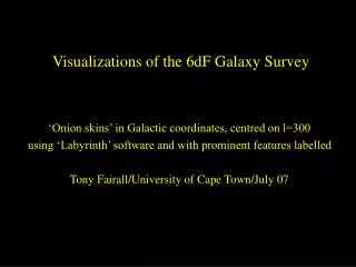
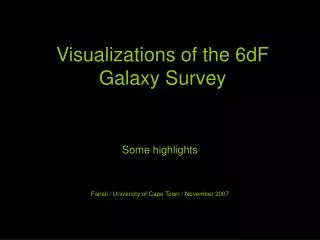
Visualizations of the 6dF Galaxy Survey. Some highlights Fairall / University of Cape Town / November 2007. Almost all galaxies (white dots) conglomerate into a network of large-scale structures, shown here as three-dimensional bodies, generated by ‘Labyrinth’ Software

E N D
Visualizations of the 6dF Galaxy Survey Some highlights Fairall / University of Cape Town / November 2007
Almost all galaxies (white dots) conglomerate into a network of large-scale structures, shown here as three-dimensional bodies, generated by ‘Labyrinth’ Software (which wraps surfaces around ‘minimal spanning trees’) 6dF reveals the bubbly texture of the Cosmos (seen here in cross section) Only about 1% of galaxies appear to lie in the voids. The void in the centre is about 60 Mpc (200 million light years across) Data used here are between -7500 and -8500 km/s in Supergalactic Z coordinates
Sometimes the structures seem almost orthogonal Data used here are between -1500 and -2500 km/s in Supergalactic Z coordinates Data absent in middle due to obscuration by the Milky Way, and top right due to northern Declinations.
‘Labyrinth’ software is used here to isolate the high-density regions. Data used here are between -2000 and -5000 km/s in Supergalactic X coordinates The 6dF Galaxy Survey finds ‘cratons’ of high density (percolated by small voids) separated by low-density regions with anaemic structures.
The ‘craton’ in the preceding slide is the previously unrecognised ‘Horologium-Canis Major’ Concentration. It is 250 Mpc (800 million light years) long Its lower end links to the Horologium Concentration
Note the void in the centre, with an empty core 100 Mpc (300 million light years) across. Its lower end also links to Horologium The Horologium-Pictor ‘craton’ (on the right) forms a parallel structure to Horologium-Canis major The data used here are between -7500 and -10000 km/s in Supergalactic X coordinates.
The width of the slide is about 100 Mpc (300 million light years) Data here are between -5000 and -7000 km/s in Supergalactic X coordinates The Horologium concentration (enlarged here) links the ‘vertical’ structures in the two previous slides
Data here are between -12000 and -15000 km/s In Supergalactic X coordinates The width of this slide is about 150 Mpc (500 million light years) Here is the more distant Telescopium Concentration
A void with ‘tessellated’ sides, seen in cross section The void is about 65 Mpc (200 million light years) across. Data shown here lie between -4000 and -5000 km/s in Supergalactic X coordinates
Alternatively the entire southern sky can be seen as a sequence of redshift shells. This sample shell shows relatively nearby structures The data used here has all 6dF redshifts between 4000 and 4999 km/s Virgo V17 V16 Hydra Void C4 Centaurus Hydra (C2) (C8) 30 0 330 300 270 240 210 Micoscopium Void (continuation of Local Void) e n t C a u r u s W a l l Pavo-Indus-Telescopium A3627 Canis Major Void C3 (N1600) LMC Aquarius Void SMC Eridanus Void Sculptor Void Cetus Sculptor Wall V31 Approx 50 Mpc (150 million light years)
Whereas this distant shell shows part of the Shapley Concentration The data used here has redshifts between 140000 and 15000 km/s V404 V415 V355 The Shapley Concentration is by far the greatest over-density in the 6dF volume. V391 V411 Leo V410 V441 V371 V348 Shapley V463 V365 V440 V341 V84 Shapley (b) V389 V386 AS0757 V477 V465 (C30) 30 0 330 300 270 240 210 Obscured by the foreground Milky Way V245 V301 C29 V88 V529 V313 V85 V277 Part of Horologium- Canis Major V230 V149 V232 V303 V264 V87 V217 Abell 3376 V200 V111 LMC SMC V36 C28 V169 V270 V272 V226 V127 V194 V287 V129 V234 V243 V131 V138 Note also the huge voids V199 V164 V125 50 Mpc (150 million light years)
A 6dF Data cube showing the Shapley Concentration RIGHT SIDE “Top” (looking -SGZ) Shapley (b) BACK FRONT Data ‘cube’ Centred at SGX = -11500 SGY=7500, SGZ=-500 100 Mpc front to back 100 Mpc left to right 70 Mpc top to bottom Shapley (a) To Earth LEFT SIDE
6dF Data cube showing the Shapley Concentration LEFT SIDE “Bottom” (looking +SGZ) Shapley (a) FRONT BACK Shapley (b) RIGHT SIDE
6dF Data cube showing the Shapley Concentration “Front” (looking –SGX)
6dF Data cube showing the Shapley Concentration FRONT “Right-hand side” (looking –SGY)
6dF Data cube showing the Shapley Concentration “Back” (looking +SGX)
6dF Data cube showing the Shapley Concentration FRONT “Left-hand side” (looking +SGY)