Subdivision I: The Univariate Setting
630 likes | 659 Vues
Subdivision I: The Univariate Setting. Peter Schröder. B-Splines (Uniform). Through repeated integration. 1. 0. 1. B 3 (x). B-Splines. Obvious properties piecewise polynomial: unit integral: non-negative: partition of unity: support:. B-Splines. Repeated convolution box function.

Subdivision I: The Univariate Setting
E N D
Presentation Transcript
Subdivision I:The Univariate Setting Peter Schröder
B-Splines (Uniform) • Through repeated integration 1 0 1 B3(x)
B-Splines • Obvious properties • piecewise polynomial: • unit integral: • non-negative: • partition of unity: • support:
B-Splines • Repeated convolution • box function x
Convolution • Reminder • definition: • translation: • dilation:
Refinability I • B-Spline refinement equation • a B-spline can be written as a linear combination of dilates and translates of itself • example • linear B-spline • and all others… 1 1/2 1/2
Refinability II • Refinement equation for B-splines • take advantage of box refinement
B-Spline Refinement • Examples
Spline Curves I • Sum of B-splines • curve as linear combination control points
Spline Curves II • Refine each B-spline in sum • example: linear B-spline 1/2 1/2 1
Spline Curves III • Refinement for curves • refine each B-spline in sum refined bases refinement of control points
Refinement of Curves • Linear operation on control points • succinctly
Refinement of Curves • Bases and control points
Subdivision Operator • Example • cubic splines
Subdivision • Apply subdivision to control points • draw successive control polygons rather than curve itself
Summary so far • Splines through refinement • B-splines satisfy refinement eq. • basis refinement corresponds to control point refinement • instead of drawing curve, draw control polygon • subdivision is refinement of control polygon
Analysis • Setup • polygon mapped to polygon • finite or (bi-)infinite, pij2Rd • subdivision operator (linear for now)
Subdivision Schemes • Some properties • affine invariance • compact support • index invariance (topologic symmetry) • local definition
Subdivision Operator • Properties • compact support • affine invariance • index invariance/symmetry
Subdivision Operator • local definition: weights depend only on local neighborhood • Terms • stationary: level independence • uniform: location independence • no boundaries (for now)
Generating Functions • Subdivision operator as convolution
Examples • Splines • linear: • quadratic: • higher order…
Examples • Quadratic splines • Chaikin’s algorithm computes new points with weights 1/4(1, 3) and 1/4(3, 1) • what happens if we change the weights?
Convergence • How much leeway do we have? • design of other subdivision rules • example: 4pt scheme • establish convergence • establish order of continuity
Analysis • Simple facts • affine invariance necessary condition for uniform convergence
Analysis • Convergence • define linear interpolant over given control points and associated parametric values (knot vector) • typically • define pointwise
Analysis • Convergence • in max/sup norm • Theorem • if then convergence of is uniform
Uniform Convergence • Proof linear spline subdivision operator
Difference Decay • Sufficient condition • continuous limit if • analysis by examining associated difference scheme
1 6 1 1/8 4 4 1/8 Example • Cubic B-splines • stencils
3 1 1 3 1/8 1/8 Example • Cubic B-splines • differences
Difference Decay • Analysis of difference scheme • construction from the subdivision scheme itself
Higher Orders • Smoothness • how to show C1? • divided differences must converge • check difference of divided differences • example • 4pt scheme
Smoothness • Consequences • 4pt scheme: decay estimate
-1 6 -1 1/8 2 2 1/8 Example • 4pt scheme • differences of divided differences
Analysis • Fundamental solution • gives basis functions
Fundamental Solution • Properties • refinement relation (why?) • support? non-zero coefficients:
So Far, So Good I • What do we know now? • regular setting • approximating • B-splines • interpolating • 4pt scheme (Deslaurier-Dubuc)
So Far, So Good II • What do we know now? • differences • continuity • differentiability • not quite general enough • current setting assumes a particular parameterization
More General Settings • Non-uniform • in spline case better curves • subdivision weights will vary • knot insertion • interpolation
4pt Scheme I • Where do the weights come from? • example of Deslaurier-Dubuc • given set of samples use interpolating polynomial to refine sample here Interpolating polynomial for 4 successive samples i-1 i i+1 i+2
4pt Scheme II • Weight computation • grind out interpolating polynomial • resulting weights: 1/16(-1, 9, 9, -1) • Deslaurier-Dubuc • generalization of same idea • higher orders yield higher continuity • tends to exhibit “ringing” (as is to be expected…)
Deslaurier-Dubuc • Local polynomial reproduction • choose sk accordingly (d =1 for 4pt) • non-uniform possible, increasing smoothness, approximation power, limit for increasing d is sync fn.
Irregular Analysis • New tools • generating functions not applicable • instead: spectral analysis (why?) • for irregular spacing only one parameter: ratio of spacing • On to spectral analysis
Analysis • We need a different approach • the subdivision matrix • a finite submatrix representative of overall subdivision operation • based on invariant neighborhoods • structure of this matrix key to understanding subdivision
j S j+1 Example • Cubic B-spline • 5 control points for 1 segment on either side of the origin
Neighborhoods • Which points influence a region? • for analysis around a point -1 1
Subdivision Matrix • Invariant neighborhood • which f(i-t) overlap the origin? • tells smoothness story
Eigen Analysis • What happens in the limit? • behavior in neighborhood of point • apply S infinitely many times… • suppose S has complete set of EVs eigen vectors control points in invariant neighborhood