PCA explained within the context of Face Recognition
670 likes | 844 Vues
PCA explained within the context of Face Recognition. Berrin Yanikoglu FENS Computer Science & Engineering Sabancı University Updated Dec. 2012. Some slides from Derek Hoiem , Lana Lazebnik, Silvio Savarese, Fei-Fei Li. Overview. Definition: Face recognition , verification, tracking…

PCA explained within the context of Face Recognition
E N D
Presentation Transcript
PCA explained within the context of Face Recognition Berrin Yanikoglu FENS Computer Science & Engineering Sabancı University Updated Dec. 2012 Some slides from Derek Hoiem, Lana Lazebnik, Silvio Savarese, Fei-Fei Li
Overview • Definition: Face recognition, verification, tracking… • Feature subspaces: PCA • Side info: Interesting findings about human face recognition
Face detection and recognition Detection Recognition “Sally”
Applications of Face Recognition • Surveillance • Digital photography • Album organization
Consumer application: iPhoto 2009 • Can be trained to recognize pets! http://www.maclife.com/article/news/iphotos_faces_recognizes_cats
Error measure With glasses Without glasses 3 Lighting conditions 5 expressions • Face Detection/Verification • False Positives (%) • False Negatives (%) • Face Recognition • Top-N rates (%) • Open/closed set problems • Sources of variations:
Face recognition • Treat pixels as a vector • Recognize face by nearest neighbor
The space of face images • When viewed as vectors of pixel values, face images are extremely high-dimensional • 100x100 image = 10,000 dimensions • Large memory and computational requirements • But very few 10,000-dimensional vectors are valid face images • We want to reduce dimensionality and effectively model the subspace of face images
Principal Component Analysis (PCA) • Pattern recognition in high-dimensional spaces • Problems arise when performing recognition in a high-dimensional space (curse of dimensionality). • Significant improvements can be achieved by first mapping the data into a lower-dimensional sub-space. where K << N. dimensionality reduction • The goal of PCA is to reduce the dimensionality of the data while retaining as much as possible of the variation present in the original dataset.
Change of basis x2 z1 Note that the vector [1 1] islonger than the vectors [1 0] or [0 1]; hence the coefficient is still 3. 3 z2 p 3 x1
Dimensionality reduction Error: x2 z2 z1 q p x1
Principal Component Analysis (PCA) • PCA allows us to compute a linear transformation that maps data from a high dimensional space to a lower dimensional sub-space. • In short, where
Principal Component Analysis (PCA) • Lower dimensionality basis • Approximate vectors by finding a basis in an appropriate lower dimensional space. (1) Higher-dimensional space representation: are the basis vectors of the N-dimensional space (2) Lower-dimensional space representation: are the basis vectors of the K-dimensional space Note: If N=K, then
Illustration for projection, variance and bases x2 z1 z2 x1
Principal Component Analysis (PCA) • Dimensionality reduction implies information loss !! • Want to preserve as much information as possible, that is: • How to determine the best lower dimensional sub-space?
Principal Components Analysis (PCA) • The projection of x on the direction of u is:z = uTx • Find the vector u such that Var(z) is maximized: Var(z) = Var(uTx) = E[ (uTx - uT m) (uTx - uT m)T] = E[(uTx – uTμ)2] //since(uTx - uT m) is a scalar = E[(uTx – uTμ)(uTx – uTμ)] = E[uT(x – μ)(x – μ)Tu] = uT E[(x – μ)(x –μ)T]u = uT∑u where ∑ = E[(x – μ)(x –μ)T] (covariance of x) In other words, we see that maximizing Var(z) is equivalent to maximizing uT∑u where u is a candidate direction we can project the data and ∑is the covariance matrix of the original data.
The next 3 slides show that the direction u that maximizes Var(z) is the eigenvectors of ∑. • You are not responsible of understanding/knowing this derivation. • The eigenvectors with the largest eigenvalue results in the largest variance. • As a result, we start picking the new basis vectors (new directions to project the data), from the eigenvectors of the cov. matrix in order (largest eigenvalue is first, then next largest etc.) • In this process, we use unit vectors to represent each direction, to remove ambiguity.
Principal Component Analysis - Advanced • Same thing, a bit more detailed: N Maximize subject to ||u||=1 Projection of data point N 1/N Covariance matrix of data
Maximize Var(z) = uT∑u subject to ||u||=1 Taking the derivative w.r.t w1,and setting it equal to 0, we get: ∑u1= αu1 u1 is an eigenvector of ∑ Choose the eigenvector with the largest eigenvalue for Var(z) to be maximum Second principal component: Max Var(z2), s.t., ||u2||=1 and it is orthogonal to u1 Similar analysis shows that,∑ u2= α u2 u2 is another eigenvector of ∑and so on. a, b:Lagrange multipliers
Maximize var(z)= • Consider the eigenvectors of Sfor which • Su = lu where u is an eigenvector of S and l is the corresponding eigenvalue. • Multiplying by uT: uTSu = uT lu = l uT u = l for ||u||=1. • => Choose the eigenvector with the largest eigenvalue.
So now that we know the new basis vectors, we need to project our old data which is centered at the origin, to find the new coordinates. • This projection is nothing but finding the individual coordinates of a point in the Cartesian space. • The point [3 4] has x-coord of 3 and y-coord of 4 because if we project onto [1 0] and [0 1] that’s what we find.
Principal Component Analysis (PCA) • Given: N data points x1, … ,xNin Rd • We want to find a new set of features that are linear combinations of original ones:u(xi) = uT(xi – µ)(µ: mean of data points) • Note that the unit vector uisin Rd(has the same dimension as the original data). Forsyth & Ponce, Sec. 22.3.1, 22.3.2
What PCA does The transformation z = WT(x – m) where the columns of W are the eigenvectors of ∑, m is sample mean, centers the data at the origin and rotates the axes If we look at our new basis vectors straight, we see it this way: a zero mean, axis-aligned distribution.
Eigenvalues of the covariance matrix - Advanced The covariance matrix is symmetrical and it can always be diagonalizedas: • where • is the column matrix consisting of • the eigenvectors ofS, • WT=W-1 • Lis the diagonal matrix whose elements are the eigenvalues ofS.
Principal Component Analysis (PCA) • Methodology • Suppose x1, x2, ..., xMare N x 1 vectors
Principal Component Analysis (PCA) • Methodology – cont.
Principal Component Analysis (PCA) • Linear transformation implied by PCA • The linear transformation RN RKthat performs the dimensionality reduction is:
How many dimensions to select? K should be << N But what should be K?
Principal Component Analysis (PCA) • How many principal components? • By using more eigenvectors, we represent more of the variation in the original data. • If we discarded all but one dimension, the new data would have lost of of the original variation in the discarded dimensions. • So, the rule used is considering to have some percentage of the original variance kept. The variance in each eigenvalue direction is lambda_i, so we sum the variance in the k direction and we require that it surpasses say 90% of the original variation.
How to choose k ? • Proportion of Variance (PoV) explained when λi are sorted in descending order • Typically, stop at PoV>0.9 • Scree graph plots of PoV vs k, stop at “elbow”
Principal Component Analysis (PCA) • What is the error due to dimensionality reduction? • We saw above that an original vector x can be reconstructed using its principal components: • It can be shown that the low-dimensional basis based on principal components minimizes the reconstruction error: • It can be shown that the error is equal to:
Effect of units in computing variance • What happens if our x1 dimension is height and x2 dimension is weight, but the height can be in cm (170cm, 190cm) or in meters (1.7m, 1.9m)… • If the unit is centimeters the variance in the x1 dimension will be larger than if we used meters.
Principal Component Analysis (PCA) • Standardization • The principal components are dependent on the units used to measure the original variables as well as on the range of values they assume. • We should always standardize the data prior to using PCA. • A common standardization method is to transform all the data to have zero mean and unit standard deviation, before applying PCA:
Eigenfaces example • Training images • x1,…,xN
Eigenfaces example Top eigenvectors: u1,…uk Mean: μ
Visualization of eigenfaces Principal component (eigenvector) uk μ + 3σkuk μ – 3σkuk
Representation and reconstruction • Face x in “face space” coordinates: =
Representation and reconstruction • Face x in “face space” coordinates: • Reconstruction: = + x µ + w1u1+w2u2+w3u3+w4u4+ …
Reconstruction P = 4 P = 200 P = 400 Eigenfaces are computed using the 400 face images from ORL face database. The size of each image is 92x112 pixels (x has ~10K dimension).
Recognition with eigenfaces Process labeled training images • Find mean µ and covariance matrix Σ • Find k principal components (eigenvectors of Σ) u1,…uk • Project each training image xi onto subspace spanned by principal components:(wi1,…,wik) = (u1T(xi – µ), … , ukT(xi – µ)) Given novel image x • Project onto subspace:(w1,…,wk) = (u1T(x– µ), … , ukT(x– µ)) • Optional: check reconstruction error x – x to determine whether image is really a face • Classify as closest training face in k-dimensional subspace ^ M. Turk and A. Pentland, Face Recognition using Eigenfaces, CVPR 1991
PCA • General dimensionality reduction technique • Preserves most of variance with a much more compact representation • Lower storage requirements (eigenvectors + a few numbers per face) • Faster matching • What are the problems for face recognition?
Limitations Global appearance method: • not robust at all to misalignment • not very robust to background variation, scale
Principal Component Analysis (PCA) • Problems • Background (de-emphasize the outside of the face – e.g., by multiplying the input image by a 2D Gaussian window centered on the face) • Lighting conditions (performance degrades with light changes) • Scale (performance decreases quickly with changes to head size) • multi-scale eigenspaces • scale input image to multiple sizes • Orientation (performance decreases but not as fast as with scale changes) • plane rotations can be handled • out-of-plane rotations are more difficult to handle