Download
1 / 22
250 likes | 606 Vues
Psychophysics of the basic sound dimensions: Frequency Resolution. Perfecto Herrera Music Perception and Cognition. Frequency resolution of our hearing system. Which is the precision of our hearing system to resolve (separate) different components (partials) of a sound stimulus?

E N D
Psychophysics of the basic sound dimensions: Frequency Resolution Perfecto Herrera Music Perception and Cognition
Frequency resolution of our hearing system Which is the precision of our hearing system to resolve (separate) different components (partials) of a sound stimulus? Implications for: -> Loudness -> Pitch -> Timbre Most of our knowledge about that comes from studies about masking
Basic elements in masking • You will hear 2 tones, one higher than the other • Count (take note of) the number of high tones that you can hear • After the pause, 2 tones are again presented • Now count the number of lower tones
Masking • The process whereby the presence of a sound (masker) raises the perceptive threshold of another sound (signal) • The magnitude that the hearing threshold is raised because of the presence of another sound. It is measured using masking decibels dBmasking = 10 log(Imasking/ I), where Imasking is the hearing threshold when the masker is present, and I is the threshold when there is no mask.
The notch in the center is an artifact of the measurement procedure, the “real” curve is smooth; the same for the second peak in the 80dB curve Masking with pure tones Effect of a sinusoidal mask of 1200 Hz @ 44, 60 i 80 dBSPL on a series of sinusoidal signals
Masking patternsfor a narrowband noise masker centred at 410 Hz. Each curve shows the elevation in threshold of a pure-tone signal as a function of signal frequency. The overall noise level in dB SPL for each curve is indicated in the figure. Data from Egan & Hake (1950). Upward spread of masking: non-linear increase of the effect for upper frequencies Linear increase with steep slopes (55-240 dB / octave)
Types of masking • Ipsilateral: masker and signal are presented in the same ear • Contralateral: the masker is presented in one ear and the signal in the opposite one (its origin is not cochlear) • Forward masking: the signal is masked by a masker that has been presented before in time (30-300ms) • Backwards masking: the masker is presented after the presentation of the signal (5ms)
Basic observations about masking • A masking sound tends to mask, first, other sounds with frequencies close to it. In order to mask further frequencies the masking sound has to be very loud. • A masking sound tends to provoke a bigger effect on upper frequencies than on lower ones. • The lower frequency a masker has, the widest range of frequencies to be masked. • The louder the masker, the widest range of frequencies to be masked.
What do masking patterns and neuron tuning curves have in common?
Auditory filters • Helmholtz (1863): • Frequency selectivity can be modelled by considering the peripheral auditory system as a bank of bandpass filters with overlapping bands • These filters are called the ‘auditory filters’ • Fletcher (1940’s): • The basilar membrane provides the basis for the auditory filters • Each location on the basilar membrane responds to a limited range of frequencies, so… • …each different point (~1mm) corresponds to a filter with a different centre frequency
Critical band • The range of frequencies around a specific one, such that in case of simultaneously listening to a tone of this frequency and a tone inside that range, the two tones are not listened to in a totally independent way • A range of frequencies over which the masking SNR remains more or less constant
Critical band • The bandwidth of the filter that determines what and how much passes a frequency channel in the transmission of information from the auditory nerve and the brain. • It determines how different frequencies are interfering mutually • The point in the basilar membrane whereby two tones of different frequencies do not interfere themselves anymore defines it. • It plays a capital role in timbre perception (fusion or separation of sounds), consonance and dissonance judgments, roughness, and masking • It plays an important role when mixing music • Width of critical band is proportional to center frequency and increases with increasing intensity (nonlinearities in cochlear transduction) • Shape does not change much with frequency • Center frequencies change according to the spectrum of the input
Measuring the critical band (Fletcher’s method) Uniform spectral density masker, increasing power as BW increases; sinusoidal signal to be masked Critical band for the test signal (4kHz) The audibility threshold of the signal raises as more power is added to the mask
Critical bandwidth Bark: Zwicker et al. (München) ERB: Moore et al. (Cambridge) What is the relation between the picture on the right and third-octave equalizers?
Equivalent Rectangular Bandwidth (ERB) • The bandwidth of a rectangular filter that has the same peak transmission as the filter of interest and passes the same total power for a white noise input. • The mean ERB of the auditory filter determined using young listeners with normal hearing and using a moderate noise level is denoted ERBN (where the subscript N denotes normal hearing) Simple formula More complex formula Computing the ERB for 400 Hz -> 24.7 * (1.748+1)= 67.87
The bark scale is a standardized scale of frequency, where each “Bark” (named after Barkhausen) constitutes one critical bandwidth. This scale can be described as approximately equal-bandwidth up to 700Hx and approximately 1/3 octave above that point • The Bark scale is often used as a frequency scale over which masking phenomenon and the shape of cochlear filters are invariant. While this is not strictly true, this represents a good first approximation
Central frequency Critical band number Upper frequency limit Lower frequency limit Central frequency Critical band number Upper frequency limit Lower frequency limit Barks and ERBs ZBark = 8.7 + 14.2 * 2 log (f/1000)
Loudness of complex sounds • Peripheral processing (filtering according to the outer and middle ear specificities) • Computation of the excitation pattern considering the masking effects (cochlea + neural firing approximation) • 3. Conversion of the excitation pattern into band-specific loudness computation. • 4. Summation of the specific band-loudness into the final loudness value • Loudness increases (additively) only when there is energy beyond the critical band
Critical bandwidth and loudness Implications for tonal music If aim is… Separately audible voices in harmony and counterpoint Then need… Separately audible partials in sonorities Physiology: Excite different hair cells with different partials Result: Separation of low tones and decreasing spacing of higher tones in chords or in simultaneous melodic lines