Probability in Methods
Probability in Methods. Summer Course Brian Healy. What have learned so far. Types of data Descriptive statistics Tables and graphs. What are we doing today?. What is probability? Empirical probability Union, Intersection, Complement Conditional probability What is a rare event?

Probability in Methods
E N D
Presentation Transcript
Probability in Methods Summer Course Brian Healy
What have learned so far • Types of data • Descriptive statistics • Tables and graphs
What are we doing today? • What is probability? • Empirical probability • Union, Intersection, Complement • Conditional probability • What is a rare event? • How to do all of these things in R
Probability • Definition: What is the chance of observing a specific event? • In repeated trials, how many would be successes? • Notation: P(Tails on next toss), P(Sunny tomorrow) • Meaning: • What is the probability that I get tails on the next toss of a coin? • What is the probability that it is going to be sunny tomorrow? • Basis of all statistical inference
Union, intersection and complement • Intersection: • Definition: probability of A AND B • Example: = Probability of having blond hair and blue eyes • Union: P(A U B) • Definition: probability of A and/or B • Example: P(Blond hair U Blue eyes) = Probability of having either blond hair, blue eyes or both • Complement: P(Ac) • Definition: probability of not A • Example: P(Blond hairc) = Probability of not having blond hair
Venn diagram Blond Hair Blue eyes • A Venn diagram is a simple graphical way to represent 2 (or more events) • The box represents all possible events • What color or colors represent: • Union of the two events? • Intersection of the two events? • Complement of the intersection? • Complement of the union? Blond hair and Blue eyes Neither blond hair or blue eyes
Conditional probability • Definition: Given that an event has occurred, what is the probability of a second event? • Conditional probability restricts the sample space by requiring that a specific event occurs • Examples: • Given that a person has blond hair, what is the probability that the person has blue eyes? • Given that it is raining today, what is the probability that it will rain tomorrow? • Given that I want the Red Sox to win, what is the probability that they will win tonight?
The mathematical definition of conditional probability is • The denominator is the probability of event B which we know has happened • The numerator of this expression is the probability that both events occur together • The multiplicative rule of probability is a simple writing of this expression. The second equality is an interesting result, which will come in handy for Bayes’ rule
Venn diagram Blond Hair Blue eyes • Suppose we are interested in the probability of having blond hair given that you have blue eyes. In terms of the Venn diagram, conditioning on having blue eyes means that we restrict our attention to people with blue eyes • Ex. The conditional probability is Blond hair and Blue eyes Neither blond hair or blue eyes
Other definitions • Mutually exclusive: Two events (A and B) that cannot occur at the same time • P(A|B) = 0 • When two events are mutually exclusive, P(A and / or B) = P(A) + P(B) • Ex. P(smoker | nonsmoker) = 0 • Exhaustive: A set of events that covers all possible events • Independent: The occurrence of event B does not affect the probability of A occurring • P(A|B) = P(A) • When two events are independent, P(A and B)=P(A|B)P(B)=P(A)P(B) • Ex. P(coin toss 2 is heads | coin toss 1 is tails) = P(coin toss 2 is heads). Note, this assumes that the coin is fair.
Venn diagram • The top diagram shows three mutually exclusive events, red hair, brown hair, and other color hair • The three events are also exhaustive because they cover all possible events • Does P(Red hair) + P(Not red hair) = 1? Why? Red hair Brown hair Any other color hair
Practice • Assume that you know the following information: P(A) = 0.7, P(B) = 0.3, P(C) = 0.5, P(A and B) = 0.21, and A and C are mutually exclusive • Answer these questions: • What is P(A|C)? • What is P(A|B)? • What can you say about events A and B? • What is P(A U B)? • What is P(Ac|C)? • What is P(Ac|B)?
Bayes’ rule • One of the most important parts of conditional probabilities is Bayes’ rule, which is used in many parts of statistics • Bayes’ rule allow exchanging the event on which you condition. This is important because it is sometimes easy to determine the conditional probability in one direction, but very difficult in the other direction. An example of this is diagnostic testing.
Diagnostic testing • When doctors give a diagnostic test, the objective is to determine how likely is it that the patient has a disease given the results of the test. In terms of math, this is P(has disease | positive test) = P(D+|T+) • If the test was perfect, the doctor would know exactly if the patient had a disease based on the test results, but tests are not perfect. In fact, test makers provide the sensitivity and specificity of the test because these are easy to measure in the laboratory • Bayes’ rule will allow use to relate the easy to measure things to determine the quantity of interest
Sensitivity: the probability of a positive test given that the patient has the disease, P(T+|D+) • Specificity: the probability of a negative test given that the patient does not have the disease, P(T-|D-) • These two are when the test was correct • False positive: the probability of a positive test given that the patient does not have the disease, P(T+|D-) • False negative: the probability of a negative test given that the patient has the disease, P(T-|D+) • Which pairs of quantities sum to 1? Why? • Why do you think it is easy to measure these quantities?
Example • A test for HIV has a sensitivity of 0.95 and a specificity of 0.9. The prevalence of HIV in the population of interest is only 0.02 • If a patient has a positive test, what is the probability that the patient actually has the disease? This is called the positive predictive value (PPV) of the test.
What is the probability that a patient does not have the disease given that the patient tests negative? This is called the negative predictive value. • As you may see, the PPV and NPV are quite low compared to the sensitivity and specificity. This is because of the small prevalence of the disease among our population. Often, public health officials will complete a two stage screen because the first stage can be used to increase the prevalence of the population and the second stage will therefore have a better PPV and NPV. • Usually, there is a trade off between sensitivity and specificity; as you increase sensitivity, you decrease specificity. The best test for a situation will depend on the type of error, false positive or false negative, that is more acceptable. For example, if you are screening for HIV among commercial sex workers, false negatives are very bad because these people are likely to have many contacts; therefore, we want to have very high sensitivity.
Parameter of interest • As you have discussed in probability, each probability distribution has parameters to describe the shape • Ex. As a teacher, I was amazed at the amount of time my students spent watching TV. Suppose the distribution of time that 7th graders watch TV is normally distributed. • What are the parameters of this distribution? • How could we estimate these?
Normal distribution-review • Continuous random variable • Range (-inf,inf) • Two parameters • Mean: m • Variance: s2 • Symmetric
Normal distribution in R • pnorm(q,mean=0,sd=1, lower.tail=T): Find the area in the lower tail below q (CDF) • You can change the parameters of the normal • dnorm(p,mean=0,sd=1, lower.tail=T): Find the value for which the CDF is equal to p • rnorm(n, mean=0, sd=1): Generates values from a N(0,1) • **Practice** • Find the value of the CDF of N(0,1) at x=0.5. • At which X is the CDF of a N(1,5) equal to 0.25?
Other distributions • dnorm allows PDF to be calculated at specific values, but not always appropriate • Binomial • pbinom, dbinom, qbinom, rbinom • Poisson • ppois, dpois, qpois, rpois • Student’s t • pt, dt, qt, rt • etc.
What if we don’t know the parameters • Often the parameters of a distribution are not known, but we would like to estimate them. • Ex. • population mean • population median • population rate
Estimation of population mean • Two types of estimates: • Point estimate: a single number estimate of the parameter of interest • Interval estimate: give an interval in which the parameter lives (next class) • You have collected one sample X1, X2,…, Xn, (independent, identically distributed) • How would you estimate the population mean?
Sample mean • The sample mean is a logical way to estimate the population mean • Is this exactly the population mean? • If you took a second sample, what would you expect about this sample mean compared to the original sample mean?
Characteristics of sample mean • Mean of sample mean: • Unbiased • Variance of sample mean: • Variance decreases as n increases
Population • In real life, you would never have the entire population, but for this example assume that we do • Load file: data<-read.table(“G:\\BIO232\\Summer\\ .dat”) • Plot a histogram of the data to see the population distribution • Find the mean and standard deviation of the population
Samples • Take 5 samples of size 10 and find the mean of each • Are the sample means equal? • What is the mean of the sample means? • What can you say about the variability of the sample means compared to the population? • Now take 5 samples of size 100 and find the mean of each
Amazing!!! • Let’s try this in an experiment… • www. • What happens as we increased the sample size? • What changes? • Why do we want a large sample size? • What is the distribution of the sample mean?
Central limit theorem • In you take a sample of size n, the distribution of the sample means are • NORMAL!!! • Mean=m • Standard deviation= • This holds true no matter the underlying population distribution!!! • So when we take a sample, we know the distribution of the sample mean
Example • Assume that we have a population with blood pressure m=80and s=10 • This distribution is not necessarily normal • If we draw a sample of size 25, what is the probability that the mean of the sample will be greater than 84?
Hints • What is the distribution of the sample mean? • What is the mean of this distribution? • What is the standard deviation of this distribution? • How can we find the probability?
Draw the picture • Always good to start with the picture
Answer • Use R • pnorm(84,mean=80,sd=2,lower.tail=F) • Use standard normal: • Mean=0, standard deviation=1 • Can standardize an normal random variable into a standard normal by subtracting the mean and dividing by standard deviation • pnorm(2, lower.tail=F)
Practice • What is the probability of being larger than 84 with a sample of size • 5? • 100? • What is the probability of being between 78 and 85 with a sample of size • 25? • 64?
Practice 2 • For a sample of size 25, what is the 90th percentile of the sample means distribution? • To complete this in R, qnorm(0.9, mean=80, sd=2)
Why is this so important • Allows hypothesis testing!!! • Definition: Comparison of a sample value to a hypothesized value to determine if the sample is significantly different than the hypothesis