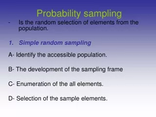
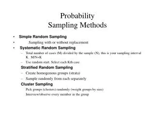
Probability Sampling Methods
Probability Sampling Methods. Simple Random Sampling Sampling with or without replacement Systematic Random Sampling Total number of cases (M) divided by the sample (N), this is your sampling interval K. M/N=K Use random start. Select each Kth case Stratified Random Sampling

Probability Sampling Methods
E N D
Presentation Transcript
ProbabilitySampling Methods • Simple Random Sampling • Sampling with or without replacement • Systematic Random Sampling • Total number of cases (M) divided by the sample (N), this is your sampling interval K. M/N=K • Use random start. Select each Kth case Stratified Random Sampling • Create homogenous groups (strata) • Sample randomly from each separately Cluster Sampling Pick groups (clusters) randomly (weight groups by size) Interview/observe every member in the group
General Rules of Probability Sampling • The larger the sample the more confidence we have in the representativeness of our sample • The more homogenous our population is the more confidence we have in the representativeness of our sample • The fraction of the population that a sample contains does not affect the sample representativeness unless the fraction is large.(less than 2%)
Rules of Probability Addition Rule The probability of either of two incompatible (mutually exclusive) events happening is the probability of the first plus the probability of the second. P(A or B)=P(A)+P(B) The sum of all the probability of all incompatible events is 1. • Multiplication Rule • The probability of two independent events happening together is the probability of the first times the probability of the second. P(A and B)=P(A)*P(B)
Probability Distributions • Imagine we flip a coin.four times Fair coin P(H)=P(T)=.5 HH • P(H and H)=.5*.5 Multiplication Rule • P(H and H and H and H)=P(HHHH)=.5*.5*.5*.5=.0625 • P(HHHT)=5*.5*.5*.5= =.0625 • P(3H, 1T in any order)= • P(HHHT)+P(HHTH)+P(HTHH)+P(THHH)=4*.0625=.25 • 0H 0 TTTT • 1H .25 TTTH, TTHT, THTT, HTTT • 2H .5 HHTT, HTHT, HTTH, THTH, TTHH, THHT • 3H .75 HHHT, HHTH, HTHH, THHH • 4H 1.0 HHHH
Imagine we take a sample of 4 students from UCSD where half of the students are Male and half Female P(M)=P(F)=.5 MM • P(M and M)=.5*.5 Multiplication Rule • P(M and M and M and M)=P(MMMM)=.5*.5*.5*.5=.0625 • P(MMMF)=5*.5*.5*.5= =.0625 • P(3M, 1F in any order)= • P(MMMF)+P(MMFM)+P(MFMM)+P(FMMM)=4*.0625=.25 • 0M 0 FFFF • 1M .25 FFFM, FFMF, FMFF, MFFF • 2M .5 MMFF, MFMF, MFFM, FMFM, FFMM, FMMF • 3M .75 MMMF, MMFM, MFMM, FMMM • 4M 1.0 MMMM
Sampling Distributions • BINOMIAL DISTRIBUTION • N = 4 P = .5 • CUMULATIVE • X P(X) PROBABILITY • 0 .06250 .06250 • .25 .25000 .31250 • .5 .37500 .68750 • .75 .25000 .93750 • 1.0 .06250 1.00000 • E(X) = .50 (Expected or most likely outcome is .50)
Sampling Distributions (cont.) • N = 10 P = .5 • CUMULATIVE • X P(X) PROBABILITY • 0 .00098 .00098 • .1 .00977 .01074 • .2 .04395 .05469 _____ • .3 .11719 .17188 | • . 4 .20508 .37695 | • .5 .24609 .62305 |-- 0.89063 • .6 .20508 .82812 | • .7 .11719 .94531 _____ | • .8 .04395 .98926 • .9 .00977 .99902 • 1.0 .00098 1.00000 • E(X) = .50
Sampling Distributions (cont.) • BINOMIAL DISTRIBUTION • N = 100 P = .5 • CUMULATIVE • X P(X) PROBABILITY • .45 .04847 .04847 • .46 .05796 .10643 • .47 .06659 .17302 • .48 .07353 .24655 • .49 .07803 .32458 • .50 .07959 .40417 • .51 .07803 .48220 • .52 .07353 .55572 • .53 .06659 .62231 • .54 .05796 .68027 • .55 .04847 .72875 • E(X) = .50
Central Limit Theorem: • 1. The sampling distribution is a normal distribution. • 2. The average of the sample averages will be the population parameter • 3. As you increase the sample size the samples will cluster closer and closer to the population parameter (less sampling error or smaller standard error).
Sampling error • Confidence level • 90%, 95% • Margin of error • Estimate + or – Multiplier*Standard Error • Standard Error: a measure of the spread of the sampling distribution • Multiplier: it depends on the level of confidence. For 95% it is 1.96, for 90% it is 1.645. • Confidence level 95% the maximum sampling error of a proportion is • N=400 ~ +- 5% • N=900 ~+- 3.3% • N=1600 ~+- 2.5% • N=6400 ~+- 1.2%
Determining Sample Size • Less error larger sample • More homogenous population smaller sample • More variables cross cutting larger sample • When weak relationships are expected large sample • Usual size over 400 between 1000 and 1500