spike-triggering stimulus features
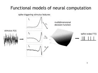
Functional models of neural computation. spike-triggering stimulus features. f 1. multidimensional decision function. x 1. stimulus X(t). f 2. spike output Y(t). x 2. f 3. x 3. Given a set of data, want to find the best reduced dimensional description.


spike-triggering stimulus features
E N D
Presentation Transcript
Functional models of neural computation spike-triggering stimulus features f1 multidimensional decision function x1 stimulus X(t) f2 spike output Y(t) x2 f3 x3
Given a set of data, want to find the best reduced dimensional description. The data are the set of stimuli that lead up to a spike, Sn(t) , where t = 1, 2, 3, …., D Variance of a random variable = < (X-mean(X))2> Covariance = < (X – mean(X))T (X – mean(X)) > Compute the difference matrix between covariance matrix of the spike-triggered stimuli and that of all stimuli Find its eigensystem to define the dimensions of interest
Eigensystem: any matrix M can be decomposed as M = U V UT , where U is an orthogonal matrix; V is a diagonal matrix, diag([l1,l2,..,lD]). Each eigenvalue has a corresponding eigenvector, the orthogonal columns of U. The value of the eigenvalue classifies the eigenvectors as belonging to column space = orthogonal basis for relevant dimensions null space = orthogonal basis for irrelevant dimensions We will project the stimuli into the column space.
This method finds an orthogonal basis in which to describe the data, and ranks each “axis” according to its importance in capturing the data. Related to principal component analysis. Functional basis set.
Example: An auditory neuron is responsible for detecting sound at a certain frequency w. Phase is not important. The appropriate “directions” describing this neuron’s relevant feature space are Cos(wt) and Sin(wt). This will describe any signal at that frequency, independent of phase: cos(A+B) = cos(A) cos(B) - sin(A) sin(B) cos(wt + f) = a cos(wt) + b sin(wt), a = cos(f), b = -sin(f). Note that a2 + b2 = 1; all such stimuli lie on a ring.
0.4 0.3 0.2 0.1 Velocity 0 -0.1 -0.2 -0.3 -0.4 150 100 50 0 Pre-spike time (ms) Modes look like local frequency detectors, in conjugate pairs (sin & cosine)… and they sum in quadrature, i.e. the decision function depends only on x2 + y2
Basic types of computation: • integrators (H1) • differentiators (retina, simple cells, single neurons) • frequency-power detectors • (complex cells, somatosensory, auditory, • retina)
Functional models of neural computation spike-triggering stimulus features f1 multidimensional decision function x1 stimulus X(t) f2 spike output Y(t) x2 f3 x3
Spike statistics Stochastic process that generates a sequence of events: point process Probability of an event at time t depends only on preceding event: renewal process All events are statistically independent: Poisson process Homogeneous Poisson: r(t) = r independent of time probability to see a spike only depends on the time you watch. PT[n] = (rT)n exp(-rT)/n! Exercise: the mean of this distribution is rT the variance of this distribution is also rT. The Fano factor = variance/mean = 1 for Poisson processes. The CV = coefficient of variation = STD/mean = 1 for Poisson Interspike interval distribution P(T) = r exp(-rT)
The Poisson model (homogeneous) Probability of n spikes in time T as function of (rate T) Poisson approaches Gaussian for large rT (here = 10)
How good is the Poisson model? Fano Factor A B Area MT Data fit to: variance = A meanB Fano factor
How good is the Poisson model? ISI analysis ISI distribution generated from a Poisson model with a Gaussian refractory period ISI Distribution from an area MT Neuron
How good is the Poisson Model? CV analysis Poisson Coefficients of Variation for a set of V1 and MT Neurons Poisson with ref. period
Interval distribution of Hodgkin-Huxley neuron driven by noise
What is the language of single cells? • What are the elementary symbols of the code? • Most typically, we think about the response as a firing rate, r(t), or a modulated • spiking probability, P(r = spike|s(t)). • We measure spike times. • Implicit: a Poisson model, where spikes are generated randomly with • local rate r(t). • However, most spike trains are not Poisson (refractoriness, internal dynamics). Fine temporal structure might be meaningful. • Consider spike patterns or “words”, e.g. • symbols including multiple spikes and the interval between • retinal ganglion cells: “when” and “how much”
Multiple spike symbols from the fly motion sensitive neuron Spike Triggered Average 2-Spike Triggered Average (10 ms separation) 2-Spike Triggered Average (5 ms)
Want to solve for K. Multiply by s(t-t’) and integrate over t: Note that we have produced terms which are simply correlation functions: Given a convolution, Fourier transform: Now we have a straightforward algebraic equation for K(w): Solving for K(t), Predicting the firing rate Let’s start with a rate response, r(t) and a stimulus, s(t). The optimal linear estimator is closest to satisfying
Going back to: Predicting the firing rate For white noise, the correlation function Css(t) = s2 d(t), So K(t) is simply Crs(t).