Download
1 / 31
350 likes | 708 Vues
Bayesian and Geostatistical Approaches to Inverse Problems. Peter K. Kitanidis Civil and Environmental Engineering Stanford University. Outline:. Important points Current Work. Inverse Problem:. Estimate functions from sparse and noisy observations;

E N D
Bayesian and Geostatistical Approaches to Inverse Problems Peter K. Kitanidis Civil and Environmental Engineering Stanford University
Outline: • Important points • Current Work
Inverse Problem: • Estimate functions from sparse and noisy observations; • The unknowns are sensitive to data gaps or flaws (Problem is ill-posed in the sense of Hadamard); • Data are insufficient to zero in on a unique solution; • Usually, it is the small-scale variability that cannot be resolved.
Cheney, M. (1997), Inverse boundary-value problems, American Scientist, 85: 448-455.
Bayesian Inference Applied to Inverse Modeling Likelihood of unknown parameter given data Posterior distribution of unknown parameter Prior distribution of unknown parameter y : measurements s : “unknown”
Bayesian Inference Applied to Inverse Modeling Information from observations Combined information (data and structure) Information about structure y : measurements s : “unknown”
How do you get the structure? • We often use an “empirical Bayes” in which the structure pdf is parameterized and inferred from the data; the approach is rigorous and robust. • Alternative interpretation: We use cross-validation. • In specific applications, we may use “geological” or other information to describe structure.
Computational cost • Reduce cost by dealing with special cases, or • Bite the bullet and use computer intensive numerical methods (MCMC, etc.)
The importance of properly weighing observations A source identification problem Identify the pumping rate at an extraction well from head observations, in a neighboring monitoring well:
Over-weighting Observations Five slides from: Kitanidis, P. K. (2007), On stochastic inverse modeling, in Subsurface Hydrology Data Integration for Properties and Processes edited by D. W. Hyndman, F. D. Day-Lewis and K. Singha, pp. 19-30, AGU, Washington, D. C.
Under-weighting Observations
The cost of computations… • Moore’s law: Cost of computations is halved every 1.5 years. Thus, between 1975 and 2006: 2^(31/1.5)=1.7E6. • $5,000 of computer usage for a project in 1975. • 1975$5,000 -- adjust for inflation -> 2006$20,000. • $20,000/1.7E6 corresponds to 1 cent worth of computational power in 2006.
METHOD—Markov Chain Monte Carlo • Based on Michalak and Kitanidis (2003 and 2004) • Use EM method on marginal distributions to find optimal parameters for structure and epistemic error. • Employ a Gibbs sampler to build a set of conditional realizations of posterior pdf. (A large enough set of conditional realizations has the same statistical properties as the actual posterior distribution.)
A problem of forensic environmental engineering PCE data at location PPC13. Measurement data and fitted concentrations resulting from the estimated boundary conditions. Michalak, A.M., and P.K. Kitanidis (2003) “A Method for Enforcing Parameter Nonnegativity in Bayesian Inverse Problems with an Application to Contaminant Source Identification,” Water Resources Research, 39(2), 1033, doi:10.1029/2002WR001480.
Location PPC13. Estimated time variation of boundary concentration at the interface between the aquifer and aquitard. The end time represents the sampling date (June 6, 1996).
PCE data at location PPC13 with non-negativity constraint. Measurement data and fitted concentrations resulting from the estimated boundary conditions.
Location PPC13 with non-negativity constraint. Estimated time variation of boundary concentration at the interface between the aquifer and aquitard. The end time represents the sampling date (June 6, 1996).
TRACER RESPONSE—Synthetic Case Tracer Input True Transfer Function Output Without Error With Error Fienen, M. N., J. Luo, and P. Kitanidis (2006), A Bayesian Geostatistical Transfer Function Approach to Tracer Test Analysis, Water Resour. Res., 42, W07426, 10.1029/2005WR004576.
Current Work • Large variance and highly nonlinear problems (Convergence of Gauss-Newton, usefulness of Fisher matrix, etc.) • Tomographic inverse problems (development of protocols, processing of large data sets.)
Current Work (cont.) • Identification of zone boundaries. • Solution methods for very large data sets. • Making tools available to users.
Identification of zone boundaries:Example • Linear tomography • Zones + small-scale variability • measurement error (2%) Four slides from the work of Michael Cardiff
We are developing… • Stochastic analysis of zone uncertainty • Merging of structural (level set) and geostatistical inverse problem concepts • Use of level sets for joint inversion
Toolbox for COMSOL Multiphysics is a commercial general purpose PDE solver. We are adding inverse-model capabilities, including adjoint-state sensitivity analysis and stochastics. See: Cardiff, M, and P. K. Kitanidis, “Efficient solution of nonlinear underdetermined inverse problems with a generalized PDE solver”, Computers and Geosciences, in review, 2007.
Our approach is: • Stochastic: (aka probabilistic or statistical): We assign a probability to every possible solution. • Bayesian: Because the Bayesian approach provides a general framework. • Geostatistical: We have adopted the best ideas from the geostatistical school. • Practical: Our methods are evolving, with particular emphasis on practicality, robustness, and computational efficiency.
For More Info See publications on the WWW: http://www.stanford.edu/group/peterk/publications.htm