Two Approaches to Bayesian Network Structure Learning

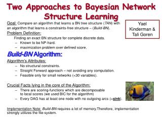
1. Two Approaches to Bayesian Network Structure Learning Yael Kinderman & Tali Goren Goal:Compare an algorithm that learns a BN tree structure (TAN) with an algorithm that learns a constraints-free structure – (Build-BN). Problem Definition: Finding an exact BN structure for complete discrete data. • Known to be NP-hard. • maximization problem over defined score. Build-BN Algorithm: Algorithm’s Attributes: • No structural constraints. • Straight Forward approach – not avoiding any computation. • Feasible only for small networks (<30 variables). Crucial Facts lying in the core of the Algorithm: • There are scoring-functions which are decomposable to local scores (we used BIC for the algorithm) • Every DAG has at least one node with no outgoing arcs (=sink). • Implementation Note:Build-BN requires a lot of memory.Therefore, implementation strongly utilizes the file-system.

2. BIC(x,vs) = Where: k iterates over all possible values of x J iterates over all possible values of Pa(x), N = number of samples Nj = number of samples where par(X)= j, Njk = “ “ “ “ “ “ “ and X=k. Algorithm’s Flow Step I: Find Local Scores: , (V = set of all variables), calculate ‘local BIC’: " Î  x V , vs ( V \ x ) All in all, n2n-1 scores are calculated in this step. Step II: Find Best Parents: , find best parents of x in the var-set. Traversing var-sets by lexicographic order (smaller to larger), Results in time complexity of O((n-1)2n-1).

3. ) Sink*(W) arg max ( skore ( W , s ) Algorithm’s Flow – cont. Step III: Find Best Sinks For each 2n var-sets we find a best sink. Let Sink*(W) be the best sinkof a var-set W. Then Sink*(W) canbe found by: = Î s W • Where: g*s(var-set) = the best set of parents for s in the var-set. • G*(var-set) = the highest scoring network for a var-set. • We traverse var-sets by lexicographic order, and use scores that were calculated in previous iterations.

4. Algorithm’s Flow – cont. Step IV:Find Best Order Best sinks immediately yield the best ordering (in reverse order). Step V: Find best network Having best order (ordi*(V)) and best parents (g*(W)) for each W V, we can find the network as following: { } | | V = * * * U ord ( V ) sin k ( V \ ord ( V ) ) i j = + 1 j i In other words: the ith var in the optimal ordering, picks best parents from the var-set that contains all the variables that are predecessors in the ordering.

5. Using the BN for Prediction • 5-fold cross validation:80% of the data used for building structure & CPDs,20% “ “ “ “ “ ‘label prediction’. • Predicting the label ‘C’ of a given sample is done using:

6. Prediction Success Rate: 0.836 Prediction Success Rate: 0.85 Test over the Famous ‘Student’ Model Testing our implementation over ‘synthetic’ data: • We simulated 300 samples according to the BN and the CPDs as were presented in class. • Prediction performed using TAN and build-BN. Build-BN result TAN result Note: In Build-BN, 4 out of 5 fold cross validation gave the above net.

7. Experimental Results Data taken from: UCI machine learning DB • Possible explanation for the last 2 results: • Zoo – only 101 instances… • Vehicle – what’s wrong with this data ?!  • Note the low in-degrees (model induced by data-sets are by nature close to trees).

8. TAN result Prediction Success Rate: 0.969 Prediction Success Rate: 0.937 Example I: CorralBuild-BN does not force‘Irrelevant’ variables to be linked into the BN Build-BN result

9. Build-BN result TAN result Prediction Success Rate: 0.844 Prediction Success Rate: 0.653 Example II – TIC TAC TOENo constraints on the structure enables better prediction References: Tomi Silander, Petri Myllymaki, HIIT. A Simple Approach for Finding the Globally Optimal Bayesian Network Structure.