Bayesian Network

1. Bayesian Network

2. Introduction • Independence assumptions • Seems to be necessary for probabilistic inference to be practical. • Naïve Bayes Method • Makes independence assumptions that are often not true • Also called Idiot Bayes Method for this reason. • Bayesian Network • Explicitly models the independence relationships in the data. • Use these independence relationships to make probabilistic inferences. • Also known as: Belief Net, Bayes Net, Causal Net, …

3. Battery Gas Start Why Bayesian Networks? • Intuitive language • Can utilize causal knowledge in constructing models • Domain experts comfortable building a network • General purpose “inference” algorithms • P(Bad Battery | Has Gas, Won’t Start) • Exact: Modular specification leads to large computational efficiencies

4. Random Variables • A random variable is a set of exhaustive and mutually exclusive possibilities. • Example: • throwing a die: • small {1,2} • medium: {3,4} • large: {5,6} • Medical data • patient’s age • blood pressure • Variable vs. Event a variable taking a value = an event.

5. Independence of Variables • Instantiation of a variable is an event. • A set of variables are independent iff all possible instantiations of the variables are independent. • Example: X: patient blood pressure {high, medium, low} Y: patient sneezes {yes, no} P(X=high, Y=yes) = P(X=high) x P(Y=yes) P(X=high, Y=no) = P(X=high) x P(Y=no) ... ... P(X=low, Y=yes) = P(X=low) x P(Y=yes) P(X=low, Y=no) = P(X=low) x P(Y=no) • Conditional independence between a set of variables holds iff the conditional independence between all possible instantiations of the variables holds.

6. Bayesian Networks: Definition • Bayesian networks are directed acyclic graphs (DAGs). • Nodes in Bayesian networks represent random variables, which is normally assumed to take on discrete values. • The links of the network represent direct probabilistic influence. • The structure of the network represents the probabilistic dependence/independence relationships between the random variables represented by the nodes.

7. Example

8. Bayesian Network: Probabilities • The nodes and links are quantified with probability distributions. • The root nodes (those with no ancestors) are assigned prior probability distributions. • The other nodes are assigned with the conditional probability distribution of the node given its parents.

9. Example Conditional Probability Tables (CPTs)

10. Noisy-OR-Gate • Exception Independence Noisy-OR-Gate—the exceptions to the causations are independent. P(E|C1, C2)=1-(1-P(E|C1))(1-P(E|C2))

11. Inference in Bayesian Networks • Given a Bayesian network and its CPTs, we can compute probabilities of the following form: P(H | E1, E2,... ... , En) where H, E1, E2,... ... , En are assignments to nodes (random variables) in the network. • Example: The probability of family-out given lights out and hearing bark: P( fo |Ø lo, hb).

12. Example: Car Diagnosis

13. MammoNet

14. Applications of Bayesian Networks

15. Application of Bayesian Network:Diagnosis

16. ARCO1: Forecasting Oil Prices

17. ARCO1: Forecasting Oil Prices

18. Semantics of Belief Networks • Two ways understanding the semantics of belief network • Representation of the joint probability distribution • Encoding of a collection of conditional independence statements

19. Y1 Y2 X Non-descendent Terminology Ancestor Parent Non-descendent Descendent

20. Three Types of Connections

21. Connection Pattern and Independence • Linear connection: The two end variables are usually dependent on each other. The middle variable renders them independent. • Converging connection: The two end variables are usually independent on each other. The middle variable renders them dependent. • Divergent connection: The two end variables are usually dependent on each other. The middle variable renders them independent.

22. D-Separation • A variable a is d-separated from b by a set of variables E if there does not exist a d-connecting path between a and b such that • None of its linear or diverging nodes is in E • For each of the converging nodes, either it or one of its descendents is in E. • Intuition: • The influence between a and b must propagate through a d-connecting path

23. If a and b are d-separated by E, then they are conditionally independent of each other given E: P(a, b | E) = P(a | E) x P(b | E)

24. Example Independence Relationships

25. Chain Rule • A joint probability distribution can be expressed as a product of conditional probabilities: P(X1, X2, ..., Xn) =P(X1) x P(X2, X1, ..., Xn | X1) =P(X1) x P(X2|X1) x P(X3, X4, ..., Xn| X1, X2) =P(X1) x P(X2|X1) x P(X3|X1,X2) x P(X4, ..., Xn|X1,X2,X3)... ... = P(X1) x P(X2|X1) x P(X3|X1, X2)x ...x P(Xn| X1, ...Xn-1) This has nothing to do with any independence assumption!

26. Compute the Joint Probability • Given a Bayesian network, let X1, X2, ..., Xn be an ordering of the nodes such that only the nodes that are indexed lower than i may have directed path to Xi. • Since the parents of Xi, d-separates Xi and all the other nodes that are indexed lower than i, P(Xi| X1, ...Xi-1)=P(Xi| parents(Xi)) This probability is available in the Bayesian network. • Therefore, P(X1, X2, ..., Xn) can be computed from the probabilities available in Beyesian network.

27. P(fo, ¬lo, do, hb, ¬bp) = ?

28. What can Bayesian Networks Compute? • The inputs to a Bayesian Network evaluation algorithm is a set of evidences: e.g., E = { hear-bark=true, lights-on=true } • The outputs of Bayesian Network evaluation algorithm are P(Xi=v | E) where Xi is an variable in the network. • For example: P(family-out=true| E) is the probability of family being out given hearing dog's bark and seeing the lights on.

29. Computation in Bayesian Networks • Computation in Bayesian networks is NP-hard. All algorithms for computing the probabilities are exponential to the size of the network. • There are two ways around the complexity barrier: • Algorithms for special subclass of networks, e.g., singly connected networks. • Approximate algorithms. • The computation for singly connected graph is linear to the size of the network.

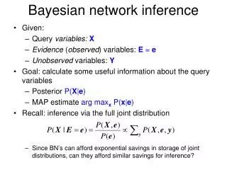
30. www.cs.cmu.edu/~awm/381/lec/bayesinfer/bayesinf.ppt Bayesian Network Inference • Inference: calculating P(X |Y ) for some variables or sets of variables X and Y. • Inference in Bayesian networks is #P-hard! Inputs: prior probabilities of .5 I1 I2 I3 I4 I5 Reduces to O P(O) must be (#sat. assign.)*(.5^#inputs) How many satisfying assignments?

31. www.cs.cmu.edu/~awm/381/lec/bayesinfer/bayesinf.ppt Bayesian Network Inference • But…inference is still tractable in some cases. • Let’s look a special class of networks: trees / forests in which each node has at most one parent.

32. www.cs.cmu.edu/~awm/381/lec/bayesinfer/bayesinf.ppt Decomposing the probabilities • Suppose we want P(Xi | E ) where E is some set of evidence variables. • Let’s split E into two parts: • Ei- is the part consisting of assignments to variables in the subtree rooted at Xi • Ei+ is the rest of it Xi

33. www.cs.cmu.edu/~awm/381/lec/bayesinfer/bayesinf.ppt Decomposing the probabilities Xi • Where: • a is a constant independent of Xi • p(Xi) = P(Xi |Ei+) • l(Xi) = P(Ei-| Xi)

34. www.cs.cmu.edu/~awm/381/lec/bayesinfer/bayesinf.ppt Using the decomposition for inference • We can use this decomposition to do inference as follows. First, compute l(Xi) = P(Ei-| Xi)for all Xi recursively, using the leaves of the tree as the base case. • If Xi is a leaf: • If Xi is in E : l(Xi) = 0 if Xi matches E, 1 otherwise • If Xi is not in E : Ei- is the null set, so P(Ei-| Xi) = 1 (constant)

35. www.cs.cmu.edu/~awm/381/lec/bayesinfer/bayesinf.ppt Quick aside: “Virtual evidence” • For theoretical simplicity, but without loss of generality, let’s assume that all variables in E (the evidence set) are leaves in the tree. • Why can we do this WLOG: Equivalent to Xi Xi Observe Xi Xi’ Observe Xi’ Where P(Xi’|Xi) =1 if Xi’=Xi, 0 otherwise

36. www.cs.cmu.edu/~awm/381/lec/bayesinfer/bayesinf.ppt Calculating l(Xi) for non-leaves Xi • Suppose Xi has one child, Xj • Then: Xj

37. www.cs.cmu.edu/~awm/381/lec/bayesinfer/bayesinf.ppt Calculating l(Xi) for non-leaves • Now, suppose Xihas a set of children, C. • Since Xid-separates each of its subtrees, the contribution of each subtree to l(Xi) is independent: where lj(Xi) is the contribution to P(Ei-| Xi)of the part of the evidence lying in the subtree rooted at one of Xi’s children Xj.

38. www.cs.cmu.edu/~awm/381/lec/bayesinfer/bayesinf.ppt We are now l-happy • So now we have a way to recursively compute all the l(Xi)’s, starting from the root and using the leaves as the base case. • If we want, we can think of each node in the network as an autonomous processor that passes a little “l message” to its parent. l l l l l l

39. www.cs.cmu.edu/~awm/381/lec/bayesinfer/bayesinf.ppt The other half of the problem • Remember, P(Xi|E) = ap(Xi)l(Xi). Now that we have all the l(Xi)’s, what about the p(Xi)’s? • p(Xi) = P(Xi |Ei+). • What about the root of the tree, Xr? In that case, Er+ is the null set, so p(Xr) = P(Xr). No sweat. Since we also know l(Xr), we can compute the final P(Xr). • So for an arbitrary Xi with parent Xp, let’s inductively assume we know p(Xp) and/or P(Xp|E). How do we get p(Xi)?

40. www.cs.cmu.edu/~awm/381/lec/bayesinfer/bayesinf.ppt Computing p(Xi) Where pi(Xp) is defined as Xp Xi

41. www.cs.cmu.edu/~awm/381/lec/bayesinfer/bayesinf.ppt We’re done. Yay! • Thus we can compute all the p(Xi)’s, and, in turn, all the P(Xi|E)’s. • Can think of nodes as autonomous processors passing l and p messages to their neighbors l l p p l l l l p p p p

42. www.cs.cmu.edu/~awm/381/lec/bayesinfer/bayesinf.ppt Conjunctive queries • What if we want, e.g., P(A, B | C) instead of just marginal distributions P(A | C) and P(B | C)? • Just use chain rule: • P(A, B | C) = P(A | C) P(B | A, C) • Each of the latter probabilities can be computed using the technique just discussed.

43. www.cs.cmu.edu/~awm/381/lec/bayesinfer/bayesinf.ppt Polytrees • Technique can be generalized to polytrees: undirected versions of the graphs are still trees, but nodes can have more than one parent

44. www.cs.cmu.edu/~awm/381/lec/bayesinfer/bayesinf.ppt Dealing with cycles • Can deal with undirected cycles in graph by • clustering variables together • Conditioning A A B C BC D D Set to 1 Set to 0

45. www.cs.cmu.edu/~awm/381/lec/bayesinfer/bayesinf.ppt Join trees • Arbitrary Bayesian network can be transformed via some evil graph-theoretic magic into a join tree in which a similar method can be employed. ABC A B C BCD BCD E D G DF F In the worst case the join tree nodes must take on exponentially many combinations of values, but often works well in practice