Part 2 of 3: Bayesian Network and Dynamic Bayesian Network
750 likes | 1.32k Vues
Part 2 of 3: Bayesian Network and Dynamic Bayesian Network. References and Sources of Figures. Part 1: Stuart Russell and Peter Norvig, Artificial Intelligence A Modern Approach , 2 nd ed., Prentice Hall, Chapter 13

Part 2 of 3: Bayesian Network and Dynamic Bayesian Network
E N D
Presentation Transcript
References and Sources of Figures • Part 1:Stuart Russell and Peter Norvig, Artificial Intelligence A Modern Approach, 2nd ed., Prentice Hall, Chapter 13 • Part 2:Stuart Russell and Peter Norvig, Artificial Intelligence A Modern Approach, 2nd ed., Prentice Hall, Chapters 14, 15 & 25Sebastian Thrun, Wolfram Burgard, and Dieter Fox, Probabilistic Robotics, Chapters 2 & 7 • Part 3:Sebastian Thrun, Wolfram Burgard, and Dieter Fox, Probabilistic Robotics, Chapter 2
Bayesian Network • A data structure to represent dependencies among variables • A directed graph in which each node is annotated with quantitative probability information
An Example of a Simple Bayesian Network Weather Cavity Toothache Catch Weather is independent of the other three variables. Toothache and Catch are conditionally independent, given Cavity.
Bayesian Network Full specifications: • A set of random variables makes up the nodes of the network • A set of directed links or arrows connects pairs of nodes. parentchild • Each node Xi has a conditional probability distribution P(Xi|Parents(Xi)) that quantifies the effect of the parents on the node • Directed acyclic graph (DAG), i.e. no directed cycles
Implementation of BN • Open source BN software: Java Bayes • Commercial BN software: MS Bayes, Netica
Teaching and Research Tools in Academic Environments GeNIe • Developed at the Decision Systems Laboratory, University of Pittsburgh • Runs only on Windows computers
An Example of Bayesian Network Burglary Lightning Alarm MaryCalls JohnCalls Demo using GeNIe
An Application of Bayesian Network Horvitz, et. al. (Microsoft Research) The Lumiere Project: Bayesian User Modeling for Inferring the Goals and Needs of Software Users ftp://ftp.research.microsoft.com/pub/ejh/lum.pdf
An Application of Bayesian Network Horvitz, et. al. (Microsoft Research) The Lumiere Project: Bayesian User Modeling for Inferring the Goals and Needs of Software Users ftp://ftp.research.microsoft.com/pub/ejh/lum.pdf
Basic Ideas • The process of change can be viewed as a series of snapshots • Each snapshot (called a time slice) describes the state of the world at a particular time • Each time slice contains a set of random variables, some of which are observable and some of which are not
State • Environments are characterized by state • Think of the state as the collection of all aspects of the robot and its environment that can impact the future
State Examples: • the robot's pose (location and orientation) • variables for the configuration of the robot's actuators (e.g. joint angles) • robot velocity and velocities of its joints • location and features of surrounding objects in the environment • location and velocities of moving objects and people • whether or not a sensor is broken, the level its battery charge
State denoted as: x xt: the state at time t
Environment measurement data • evidence • information about a momentary state of the environment • Examples: • camera images • range scans
Environment measurement data Denoted as: z zt: the measurement data at time t denotes the set of all measurements acquired from time t1to time t2
Control data • convey information regarding change of state in the environment • related to actuation • Examples: • velocity of a robot (suggests the robot's pose after executing a motion command) • odometry (measure of the effect of a control action)
Control data Denoted as: u ut: the change of state in the time interval (t-1;t] denotes a sequence of control data from time t1to time t2
Scenario • a mobile robot uses its camera to detect the state of the door (open or closed) • camera is noisy: • if the door is in fact open: • the probability of detecting it open is 0.6 • if the door is in fact closed: • the probability of detecting it closed is 0.8
Scenario • the robot can use its manipulator to push open the door • if the door is in fact closed: • the probability of robot opening it is 0.8
Scenario • At time t0, the probability of the door being open is 0.5 • Suppose at t1 the robot takes no control action but it senses an open door, what is the probability of the door is open?
Scenario • Using Bayes Filter, we will see that: • at time t1 the probability of the door is open is: • 0.75 after taking a measurement • at time t2 the probability of the door is open is • ~0.984 after the robot pushes open the door and takes another measurement
DBN with Evolution of States, Controls, and Measurements for the Mobile Robot Example xt : state of the door (open or closed) at time t ut: control data (robot's manipulator pushes open or does nothing) at time t zt : evidence or measurement by sensors at time t
Basic Idea of the Algorithm of Bayes Filter Bayes_filter(bel(xt-1), ut, zt): for all xt do endfor return bel(xt) Predict xt after exerting ut Update belief of xt after making a measurement zt
The subsequent slides explain how the Bayes' rule is applied in this filter.
Basic Inference Tasks in Probabilistic Reasoning • Filtering or monitoring • Prediction • Smoothing or hindsight • Most likely explanation
Filtering, or monitoring • The task of computing the belief state—the posterior distribution over the current state, given all evidence to date • i.e. compute P(Xt|z1:t)
Prediction • The task of computing the posterior distribution over the future state, given all evidence to date • i.e. compute P(Xt+k|z1:t), for some k > 0or P(Xt+1|z1:t) for one-step prediction
Smoothing, or hindsight • The task of computing the posterior distribution over the past state, given all evidence to date • i.e. compute P(Xk|z1:t), for some 0 k < t
Most likely explanation • Given a sequence of observations, we want to find the sequence of states that is most likely to have generated those observations • i.e. compute
Review Bayes' rule
Review Conditioning For any sets of variables Y and Z, Read as: Y is conditioned on the variable Z. Often referred to as Theorem of total probability.
DBN with Evolution of States and Measurements—To be used in the explanation of filtering and prediction tasks in the subsequent slides xt : state of the door (open or closed) at time t zt : evidence or measurement by sensors at time t
The Task of Filtering • To update the belief state • By computing: from the current state
The Task of Filtering b c a a b c b c
The Task of Filtering The probability distribution of the state at t+1, given the measurements (evidence) to date i.e. it is a one-step prediction for the next state
The Task of Filtering By conditioning on the current state xt, this term becomes:
The Task of Filtering • To update the belief state • By computing: from the current state
The Task of Filtering The robot's belief state: The posterior over the state variables X at time t+1 is calculated recursively from the corresponding estimate one time step earlier
The Task of Filtering Most modern localization algorithms use one of two representations of the robot's belief: Kalman filter and particle filter called Monte Carol localization (MCL).