Bayesian Networks

Bayesian Networks October 9, 2008 Sung-Bae Cho

Agenda • Bayesian Network • Introduction • Inference of Bayesian Network • Modeling of Bayesian Network • Bayesian Network Application • Bayesian Network Application Example • Life Log Application Example • Summary & Review

5 7 Probabilities • Probability distribution P(X|x) • X is a random variable • Discrete random variable: Finite set of possible outcomes • Continuous random variable: Probability distribution (density function) over continuous values • xis background state of information X binary:

Rules of Probability • Product Rule • Marginalization • Bayes Rule X binary:

Rules of Probability • Chain rule of probability

The Joint Distribution • Recipe for making a joint distribution of M variables • Make a truth table listing all combinations of values of your variables • For each combination of values, say how probable it is

Using the Joint • Once you have the joint distribution, you can ask for the probability of any logical expression involving your attribute

Using the Joint

Inference with Joint

Inference with the Joint

Good news Once you have a joint distribution, you can ask important questions about stuff that involves a lot of uncertainty Bad news Impossible to create for more than about ten attributes because there are so many numbers needed when you build them Joint Distributions

Bayesian Networks • In general • P(X1, … Xn) needs at least 2n – 1numbers to specify the joint probability • Exponential storage and inference • Overcome the problem of exponential size by exploiting conditional independence REAL Joint Probability Distribution (2n-1 numbers) Graphical Representation of Joint Probability Distribution (Bayesian Network) Conditional Independence (Domain knowledge or Derived from data)

P(A) P(S) Visit to Asia Smoking P(L|S) P(T|A) P(B|S) Lung Cancer Tuberculosis Bronchitis CPD: T L B D=0 D=1 0 0 0 0.1 0.9 0 0 1 0.7 0.3 0 1 0 0.8 0.2 0 1 1 0.9 0.1 ... P(C|T,L) P(D|T,L,B) Chest X-ray Dyspnoea Conditional Independencies Efficient Representation Bayesian Networks? P(A, S, T, L, B, C, D) = P(A) P(S) P(T|A) P(L|S) P(B|S) P(C|T,L) P(D|T,L,B) [Lauritzen & Spiegelhalter, 95]

Bayesian Networks? • Structured, graphical representation of probabilistic relationships between several random variables • Explicit representation of conditional independencies • Missing arcs encode conditional independence • Efficient representation of joint pdf (probabilistic distribution function) • Allows arbitrary queries to be answered • P(lung cancer=yes | smoking=no, dyspnoea=yes)=?

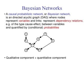
Bayesian Networks? • Also called belief networks, and (directed acyclic) graphical models • Bayesian network • Directed acyclic graph • Nodes are variables (discrete or continuous) • Arcs indicate dependence between variables • Conditional Probabilities (local distributions)

P( S=no) 0.80 P( S=light) 0.15 P( S=heavy) 0.05 Smoking= no light heavy P( C=none) 0.96 0.88 0.60 P( C=benign) 0.03 0.08 0.25 P( C=malig) 0.01 0.04 0.15 Bayesian Networks Smoking Cancer

Product Rule • P(C,S) = P(C|S) P(S) P(Smoke) P(Cancer)

Cancer= none benign malignant P( S=no) 0.821 0.522 0.421 P( S=light) 0.141 0.261 0.316 P( S=heavy) 0.037 0.217 0.263 Bayes Rule

Missing Arcs Represent Conditional Independence Start Battery Engine Turns Over Start and Battery are independent, given Engine Turns Over General product (chain) rule for Bayesian networks

Age Gender Exposure to Toxics Smoking Cancer Serum Calcium Lung Tumor Bayesian Network

Bayesian Network Knowledge Engineering • Objective: Construct a model to perform a defined task • Participants: Collaboration between domain expert and BN modeling expert • Process: iterate until “done” • Define task objective • Construct model • Evaluate model

The KE Process • What are the variables? • What are their values/states? • What is the graph structure? • What is the local model structure? • What are the parameters (Probabilities)? • What are the preferences (utilities)?

The Knowledge Acquisition Task • Variables: • collectively exhaustive, mutually exclusive values • clarity test: value should be knowable in principle • Structure • if data available, can be learned • constructed by hand (using “expert” knowledge) • variable ordering matters: causal knowledge usually simplifies • Probabilities • can be learned from data • second decimal usually does not matter; relative probabilities • sensitivity analysis

What are the Variables? • “Focus” or “query” variables • Variables of interest • “Evidence” or “Observation” variables • What sources of evidence are available? • “Context” variables • Sensing conditions, background causal conditions • Start with query variables and spread out to related variables

What are the Values/States? • Variables/values must be exclusive and exhaustive • Naive modelers sometimes create separate (often Boolean) variables for different states of the same variable • Types of variables • Binary (2-valued, including Boolean) • Qualitative • Numeric discrete • Numeric continuous • Dealing with infinite and continuous domains • Some BN software requires that continuous variables be discretized • Discretization should be based on differences in effect on related variables (i.e., not just be even sized chunks)

Values versus Probabilities Risk of Smoking Smoking What is a variable? • Collectively exhaustive, mutually exclusive values Error Occurred No Error

What is the Graph Structure? • Goals in specifying graph structure • Minimize probability elicitation: fewer nodes, fewer arcs, smaller state spaces • Maximize fidelity of model • Sometimes requires more nodes, arcs, and states • Tradeoff between more accurate model and cost of additional modeling • Too much detail can decrease accuracy

Inference • We now have compact representations of probability distributions: Bayesian Networks • Network describes a unique probability distribution P • How do we answer queries about P? • We use inference as a name for the process of computing answers to such queries

Inference - The Good & Bad News • We can do inference • We can compute any conditional probability • P( Some variables | Some other variable values ) • The sad, bad news • Conditional probabilities by enumerating all matching entries in the joint are expensive: • Exponential in the number of variables • Sadder and worse news • General querying of Bayesian networks is NP-complete • Hardness does not mean we cannot solve inference • It implies that we cannot find a general procedure that works efficiently for all networks • For particular families of networks, we can have provably efficient procedures

Example M H G S J 23JPComputation 24 JP computation

Queries: Likelihood • There are many types of queries we might ask. • Most of these involve evidence • Evidence e is an assignment of values to a set E variables in the domain • Without loss of generality E= { Xk+1, …, Xn} • Simplest query: compute probability of evidence • This is often referred to as computing the likelihood of the evidence

Queries • Often we are interested in the conditional probability of a variable given the evidence • This is the a posteriori belief in X, given evidence e • A related task is computing the term P(X, e) • i.e., the likelihood of e and X = x for values of X • we can recover the a posteriori belief by

A Posteriori Belief This query is useful in many cases: • Prediction: what is the probability of an outcome given the starting condition • Target is a descendent of the evidence • Diagnosis: what is the probability of disease/fault given symptoms • Target is an ancestor of the evidence • As we shall see, the direction between variables does not restrict the directions of the queries • Probabilistic inference can combine evidence form all parts of the network

Approaches to Inference • Exact inference • Inference in Simple Chains • Variable elimination • Clustering / join tree algorithms • Approximate inference • Stochastic simulation / sampling methods • Markov chain Monte Carlo methods • Mean field theory

Inference in Simple Chains X1 X2 • How do we compute P(X2)? • How do we compute P(X3)? • we already know how to compute P(X2)... X1 X2 X3

Xn X1 X2 X3 Inference in Simple Chains How do we compute P(Xn)? • Compute P(X1), P(X2), P(X3), … • We compute each term by using the previous one • Complexity: • Each step costs operations • Compare to naïve evaluation, that requires summing over joint values of n-1 variables

E A B C D Elimination in Chains

E E A A B B C C D D Elimination in Chains X X X

Variable Elimination General idea: • Write query in the form • Iteratively • Move all irrelevant terms outside of innermost sum • Perform innermost sum, getting a new term • Insert the new term into the product

Stochastic Simulation • Suppose you are given values for some subset of the variables, G, and want to infer values for unknown variables, U • Randomly generate a very large number of instantiations from the BN • Generate instantiations for all variables – start at root variables and work your way “forward” • Only keep those instantiations that are consistent with the values for G • Use the frequency of values for U to get estimated probabilities • Accuracy of the results depends on the size of the sample (asymptotically approaches exact results)

Markov Chain Monte Carlo Methods • So called because • Markov chain – each instance generated in the sample is dependent on the previous instance • Monte Carlo – statistical sampling method • Perform a random walk through variable assignment space, collecting statistics as you go • Start with a random instantiation, consistent with evidence variables • At each step, for some non-evidence variable, randomly sample its value, consistent with the other current assignments • Given enough samples, MCMC gives an accurate estimate of the true distribution of values

data-based Why Learning knowledge-based (expert systems) • Answer Wizard, Office 95, 97, & 2000 • Troubleshooters, Windows 98 & 2000 • Causal discovery • Data visualization • Concise model of data • Prediction

Why Learning? • Knowledge acquisition is bottleneck • Knowledge acquisition is an expensive process • Often we don’t have an expert • Data is cheap • Amount of available information growing rapidly • Learning allows us to construct models from raw data • Conditional independencies & graphical language capture structure of many real-world distributions • Graph structure provides much insight into domain • Allows “knowledge discovery” • Learned model can be used for many tasks • Supports all the features of probabilistic learning • Model selection criteria • Dealing with missing data & hidden variables

Truth Earthquake Earthquake Alarm Set AlarmSet Burglary Burglary Earthquake Alarm Set Burglary Sound Sound Sound Why Struggle for Accurate Structure? • Cannot be compensated by accurate fitting of parameters • Also misses causality and domain structure • Increases the number of parameters to be fitted • Wrong assumptions about causality and domain structure Adding an arc Missing an arc

X2 X1 X3 X4 X5 X6 X7 X8 X9 Learning Bayesian Networks from Data Bayesian networks data Bayesian network learner … … + Prior/expert information

Learning Bayesian Networks

Two Types of Methods for Learning BNs • Constraint based • Finds a Bayesian network structure whose implied independence constraints “match” those found in the data • Scoring methods (Bayesian, MDL, MML) • Find the Bayesian network structure that can represent distributions that “match” the data (i.e. could have generated the data) • Practical considerations • The number of possible BN structures is super exponential in the number of variables. • How do we find the best graph(s)?

Approaches to Learning Structure • Constraint based • Perform tests of conditional independence • Search for a network that is consistent with the observed dependencies and independencies • Pros & Cons • Intuitive, follows closely the construction of BNs • Separates structure learning from the form of the independence tests • Sensitive to errors in individual tests • Computationally hard

Bayesian Networks