Bayesian Belief Network
Bayesian Belief Network. The decomposition of large probabilistic domains into weakly connected subsets via conditional independence is one of the most important developments in the recent history of AI This can work well, even the assumption is not true!. v NB. Naive Bayes assumption:


Bayesian Belief Network
E N D
Presentation Transcript
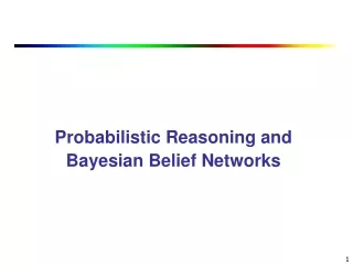
The decomposition of large probabilistic domains into weakly connected subsets via conditional independence is one of the most important developments in the recent history of AI • This can work well, even the assumption is not true!
vNB • Naive Bayes assumption: • which gives
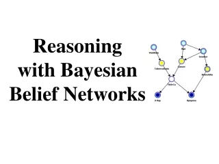
Bayesian networks • Conditional Independence • Inference in Bayesian Networks • Irrelevant variables • Constructing Bayesian Networks • Aprendizagem Redes Bayesianas • Examples - Exercisos
Naive Bayes assumption of conditional independence too restrictive • But it's intractable without some such assumptions... • Bayesian Belief networks describe conditional independence among subsets of variables • allows combining prior knowledge about (in)dependencies amongvariables with observed training data
Bayesian networks • A simple, graphical notation for conditional independence assertions and hence for compact specification of full joint distributions • Syntax: • a set of nodes, one per variable • a directed, acyclic graph (link ≈ "directly influences") • a conditional distribution for each node given its parents: P (Xi | Parents (Xi)) • In the simplest case, conditional distribution represented as a conditional probability table (CPT) giving the distribution over Xi for each combination of parent values
Y Z P Bayesian Networks • Bayesian belief network allows a subset of the variables conditionally independent • A graphical model of causal relationships • Represents dependency among the variables • Gives a specification of joint probability distribution • Nodes: random variables • Links: dependency • X,Y are the parents of Z, and Y is the parent of P • No dependency between Z and P • Has no loops or cycles X
Conditional Independence • Once we know that the patient has cavity we do not expect the probability of the probe catching to depend on the presence of toothache • Independence between a and b
Example • Topology of network encodes conditional independence assertions: • Weather is independent of the other variables • Toothache and Catch are conditionally independent given Cavity
Bayesian Belief Network: An Example Family History Smoker (FH, ~S) (~FH, S) (~FH, ~S) (FH, S) LC 0.7 0.8 0.5 0.1 LungCancer Emphysema ~LC 0.3 0.2 0.5 0.9 The conditional probability table for the variable LungCancer: Shows the conditional probability for each possible combination of its parents PositiveXRay Dyspnea Bayesian Belief Networks
Example • I'm at work, neighbor John calls to say my alarm is ringing, but neighbor Mary doesn't call. Sometimes it's set off by minor earthquakes. Is there a burglar? • Variables: Burglary, Earthquake, Alarm, JohnCalls, MaryCalls • Network topology reflects "causal" knowledge: • A burglar can set the alarm off • An earthquake can set the alarm off • The alarm can cause Mary to call • The alarm can cause John to call
Belief Networks Earthquake Burglary P(B) 0.001 P(E) 0.002 Burg. Earth. P(A) t t .95 t f .94 f t .29 f f .001 Alarm JohnCalls MaryCalls A P(M) t .7 f .01 A P(J) t .90 f .05
Compactness • A CPT for Boolean Xi with k Boolean parents has 2k rows for the combinations of parent values • Each row requires one number p for Xi = true(the number for Xi = false is just 1-p) • If each variable has no more than k parents, the complete network requires O(n · 2k) numbers • I.e., grows linearly with n, vs. O(2n) for the full joint distribution • For burglary net, 1 + 1 + 4 + 2 + 2 = 10 numbers (vs. 25-1 = 31)
Inference in Bayesian Networks • How can one infer the (probabilities of) values of one or more network variables, given observed values of others? • Bayes net contains all information needed for this inference • If only one variable with unknown value, easy to infer it • In general case, problem is NP hard
Example • In the burglary network, we migth observe the event in which JohnCalls=true and MarryCalls=true • We could ask for the probability that the burglary has occured • P(Burglary|JohnCalls=ture,MarryCalls=true)
Normalization • X is the query variable • E evidence variable • Y remaining unobservable variable • Summation over all possible y (all possible values of the unobservable varables Y)
P(Burglary|JohnCalls=ture,MarryCalls=true) • The hidden variables of the query are Earthquake and Alarm • For Burglary=true in the Bayesain network
To compute we had to add four terms, each computed by multipling five numbers • In the worst case, where we have to sum out almost all variables, the complexity of the network with n Boolean variables is O(n2n)
P(b) is constant and can be moved out, P(e) term can be moved outside summation a • JohnCalls=true and MarryCalls=true, the probability that the burglary has occured is aboud 28%
Variable elimination algorithm • Eliminate repeated calculation • Dynamic programming
Irrelevant variables • (X query variable, E evidence variables)
Complexity of exact inference • The burglary network belongs to a family of networks in which there is at most one undiracted path between tow nodes in the network • These are called singly connected networks or polytrees • The time and space complexity of exact inference in polytrees is linear in the size of network • Size is defined by the number of CPT entries • If the number of parents of each node is bounded by a constant, then the complexity will be also linear in the number of nodes
For multiply connected networks variable elimination can have exponentional time and space complexity
Constructing Bayesian Networks • A Bayesian network is a correct representation of the domain only if each node is conditionally independent of its predecessors in the ordering, given its parents P(MarryCalls|JohnCalls,Alarm,Eathquake,Bulgary)=P(MaryCalls|Alarm)
Conditional Independence relations in Bayesian networks • The toopological semantics is given either of the spqcifications of DESCENDANTS or MARKOV BLANKET
Example • JohnCalls is indipendent of Burglary and Earthquake given the value of Alarm
Example • Burglary is indipendent of JohnCalls and MaryCalls given Alarm and Earthquake
Constructing Bayesian networks • 1. Choose an ordering of variables X1, … ,Xn • 2. For i = 1 to n • add Xi to the network • select parents from X1, … ,Xi-1 such that P (Xi | Parents(Xi)) = P (Xi | X1, ... Xi-1) This choice of parents guarantees: P (X1, … ,Xn) = πni =1P (Xi | X1, … , Xi-1) (chain rule) = πni =1P (Xi | Parents(Xi)) (by construction)
The compactness of Bayesian networks is an example of locally structured systems • Each subcomponent interacts directly with only bounded number of other components • Constructing Bayesian networks is difficult • Each variable should be directly influenced by only a few others • The network topology reflects thes direct influences
Example • Suppose we choose the ordering M, J, A, B, E P(J | M) = P(J)?
Example • Suppose we choose the ordering M, J, A, B, E P(J | M) = P(J)? No P(A | J, M) = P(A | J)?P(A | J, M) = P(A)? No P(B | A, J, M) = P(B | A)? P(B | A, J, M) = P(B)?
Example • Suppose we choose the ordering M, J, A, B, E P(J | M) = P(J)? No P(A | J, M) = P(A | J)?P(A | J, M) = P(A)? No P(B | A, J, M) = P(B | A)? Yes P(B | A, J, M) = P(B)? No P(E | B, A ,J, M) = P(E | A)? P(E | B, A, J, M) = P(E | A, B)?
Example • Suppose we choose the ordering M, J, A, B, E P(J | M) = P(J)? No P(A | J, M) = P(A | J)?P(A | J, M) = P(A)? No P(B | A, J, M) = P(B | A)? Yes P(B | A, J, M) = P(B)? No P(E | B, A ,J, M) = P(E | A)? No P(E | B, A, J, M) = P(E | A, B)? Yes
Example contd. • Deciding conditional independence is hard in noncausal directions • (Causal models and conditional independence seem hardwired for humans!) • Network is less compact: 1 + 2 + 4 + 2 + 4 = 13 numbers needed • Some links represent tenous relationship that require difficult and unnatural probability judgment, such the probability of Earthquake given Burglary and Alarm
Aprendizagem Redes Bayesianas • Como preencher as entradas numa Tabela de Probabilidade Condicional 1º Caso: Se a estrutura da rede bayesiana fôr conhecida, e todas as variavéis podem ser observadas do conjunto de treino. Então: Entrada (i,j) = utilizando os valores observados no conjunto de treino 2º Caso: Se a estrutura da rede bayesiana fôr conhecida, e algumas das variavéis não podem ser observadas no conjunto de treino. Então utiliza-se método do algoritmo do gradiente ascendente
Exemplo 1º caso Family History Smoker • Person FH S E LC PXRay D • P1 Sim Sim Não Sim + Sim • P2 Sim Não Não Sim - Sim • P3 Sim Não Sim Não + Não • P4 Não Sim Sim Sim - Sim • P5 Não Sim Não Não + Não • P6 Sim Sim ? ? ? ? LungCancer Emphysema (FH, S) (FH, ~S) (~FH, S) (~FH, ~S) P(LC = Sim \ FH=Sim, S=Sim) =0.5 LC … 0.5 … … ~LC … … … …
Exemplo 2º caso • Person FH S E LC PXRay D • P1 --- Sim --- Sim + Sim • P2 --- Não --- Sim - Sim • P3 --- Não --- Não + Não • P4 --- Sim --- Sim - Sim • P5 --- Sim --- Não + Não • P6 Sim Sim ? ? ? ? • Suppose structure known, variables partially observable • Similar to training neural network with hidden units • In fact, can learn network conditional probability tables using gradient ascent
Summary • Bayesian networks provide a natural representation for (causally induced) conditional independence • Topology + CPTs = compact representation of joint distribution • Generally easy for domain experts to construct