Download

1 / 13
130 likes | 181 Vues
Explore the basics of Bayesian Belief Networks (BBN) with a simple example of predicting late arrivals at work due to train strikes. Learn about BBN construction, causal relations, joint probabilities, marginal distributions, and conditional probabilities using a directed acyclic graph.

E N D
Lecture onBayesian Belief Networks(Basics) Patrycja Gradowska Open Risk Assessment Workshop Kuopio, 2009
Lecture contents • Brief introduction to BBN and example • Definition of BBN • Purpose of BBN • Construction of BBN • Concluding remarks
A simple example Problem: Two colleagues Norman and Martin live in the same city, work together, but come to work by completely different means - Norman usually comes by train while Martin always drives. The railway workers go on strike sometimes. Goal: We want to predict whether Norman and Martin will be late for work.
A simple example Two causal relations: • Strike of the railway can cause Norman to be late • Strike of the railway can cause Martin to be late IMPORTANT: These relations are NOT absolute!! Strike of the railway does NOT guarantee that Norman and Martin will be late for sure.It ONLY increases the probability (chance) of lateness.
What is Bayesian Belief Network (BBN)? Bayesian Belief Network (BBN) is a directed acyclic graph associated with a set of conditional probability distributions. BBN is a set of nodes connected by directed edges in which: • nodes represent discrete or continuous random variables in the problem studied, • directed edges represent direct or causal relationships between variables and do not form cycles, • each node is associated with a conditional probability distribution which quantitatively expresses the strength of the relationship between that node and its parents.
Train Strike (TS) Norman late (NL) Martin late (ML) BBN for late-for-work example 3 discrete (Yes/No) variables
Bayesian Belief Network: gives the intuitive representation of the problem that is easily understood by non-experts incorporates uncertainty related to the problem and also allows to calculate probabilities of different scenarios (events) relevant to the problem and to predict consequences of these scenarios What do we need BBNs for?
… P(ML = Y, NL = Y, TS = N) P(ML = Y, NL = N, TS = N) P(ML = m, NL = n, TS = t) P(ML,NL,TS) = P(ML|TS)∙P(NL|TS)∙P(TS) - joint distribution BBN for late-for-work example • joint probability P(ML = Y, NL = Y,TS = N) = = P(ML = Y|TS = N)∙P(NL = Y|TS = N)∙P(TS = N) = 0.5 ∙ 0.1 ∙ 0.9 = 0.045
P(ML = Y, NL = Y) BBN for late-for-work example - marginal probability - marginal distribution (marginalization) P(ML = Y, NL = Y) = P(ML = Y, NL = Y, TS = t) = = P(ML = Y, NL = Y,TS = Y) + P(ML = Y,NL = Y,TS = N) = 0.048 + 0.045 = 0.093
P(NL = Y) BBN for late-for-work example - marginal probability - marginal distribution (marginalization) OR easier P(NL = Y) = P(ML = m, NL = Y, TS = t) = = P(ML = Y, NL = Y, TS = Y) + P(ML = N,NL = Y, TS = N) + + P(ML = N, NL = Y, TS = Y) + P(ML = Y, NL = Y, TS = N) = 0.048 + 0.045 + 0.032 + 0.045 = 0.17 P(NL = Y) = P(ML = m, NL = Y) = = P(ML = Y, NL = Y) + P(ML = N,NL = Y) = = 0.093 + 0.077 = 0.17
P(NL = Y| TS = Y)·P(TS = T) P(ML = Y| NL = Y) P(ML | NL) P(ML = Y| NL = Y) = = = 0.093 / 0.17 = 0.5471 P(ML = Y, NL = Y) P(NL = Y) P(TS = Y| NL = Y) = = = 0.08 / 0.17 = 0.471 > P(TS = T) = 0.1 P(NL = Y) BBN for late-for-work example - conditional probability - Bayes’ Theorem - conditional distribution
Building and quantifying BBN • Identification and understanding of the problem (purpose, scope, boundaries, variables) • Identification of relationships between variables and determination of the graphical structure of the BBN • Verification and validation of the structure • Quantification of conditional probability distributions • Verification and validation of the model – test runs • Analysis of the problem via conditionalization process NOT easy in practice
Additional remarks on BBNs • there are other BBNs in addition to discrete ones, i.e. continuous BBNs, mixed discrete-continuous BBNs • BBNs are not only about causal relations between variables, they also capture probabilistic dependencies and can model mathematical (functional) relationships • BBNs can be really large and complex • but once the right BBN is built the analysis of the problem is fun and simple using available BBN software, e.g. Netica, Hugin, UniNet