Download
1 / 22
220 likes | 250 Vues
Chapter 12 Probabilistic Reasoning and Bayesian Belief Networks. Chapter 12 Contents. Probabilistic Reasoning Joint Probability Distributions Bayes’ Theorem Simple Bayesian Concept Learning Bayesian Belief Networks The Noisy-V Function Bayes’ Optimal Classifier The Naïve Bayes Classifier

E N D
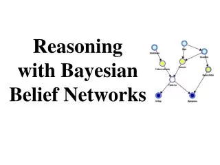
Chapter 12 Probabilistic Reasoning and Bayesian Belief Networks
Chapter 12 Contents • Probabilistic Reasoning • Joint Probability Distributions • Bayes’ Theorem • Simple Bayesian Concept Learning • Bayesian Belief Networks • The Noisy-V Function • Bayes’ Optimal Classifier • The Naïve Bayes Classifier • Collaborative Filtering
Probabilistic Reasoning • Probabilities are expressed in a notation similar to that of predicates in FOPC: • P(S) = 0.5 • P(T) = 1 • P(¬(A Λ B) V C) = 0.2 • 1 = certain; 0 = certainly not
Conditional Probability • Conditional probability refers to the probability of one thing given that we already know another to be true: • This states the probability of B, given A.
Conditional Probability • Note that P(A|B) ≠ P(B|A) • P(R/\S) = 0.01 • P(S) = 0.1 • P(R) = 0.7
Conditional Probability • Conditional probability refers to the probability of one thing given that we already know another to be true: P(A \/ B) = P(A) + P(B) – P(A /\ B) P(A /\ B) = P(A) * p(B) if A and B are independent events.
Joint Probability Distributions • A joint probability distribution represents the combined probabilities of two or more variables. • This table shows, for example, that P (A Λ B) = 0.11 P (¬A Λ B) = 0.09 • Using this, we can calculate P(A): P(A) = P(A Λ B) + P(A Λ ¬B) = 0.11 + 0.63 = 0.74
Bayes’ Theorem • Bayes’ theorem lets us calculate a conditional probability: • P(B) is the prior probability of B. • P(B | A) is the posterior probability of B.
Baye’s Thm • P(A/\B) = P(A|B) P(B) dependent events • P(A/\B) = P(B /\ A) = P(B|A) P(A) • P(A|B) P(B) = P(B|A) P(A) P(A|B) P(B) • P(B|A) = ------------ P(A)
Simple Bayesian Concept Learning (1) • P (H|E) is used to represent the probability that some hypothesis, H, is true, given evidence E. • Let us suppose we have a set of hypotheses H1…Hn. • For each Hi • Hence, given a piece of evidence, a learner can determine which is the most likely explanation by finding the hypothesis that has the highest posterior probability.
Simple Bayesian Concept Learning (2) • In fact, this can be simplified. • Since P(E) is independent of Hi it will have the same value for each hypothesis. • Hence, it can be ignored, and we can find the hypothesis with the highest value of: • We can simplify this further if all the hypotheses are equally likely, in which case we simply seek the hypothesis with the highest value of P(E|Hi). • This is the likelihood of E given Hi.
Example • If high temp (A), have cold (B) – 80% • P(A|B) = 0.8 • Suppose 1 in 10,000 have cold • Suppose 1 in 1,000 have high temp • P(A) = 0.001 P(B) = 0.0001 • P(B|A) = {P(A|B)*P(B)}/P(A) • = 0.008 8 chances in 1000 that you have a cold when having a high temp.
Bayesian Belief Networks (1) • A belief network shows the dependencies between a group of variables. • If two variables A and B are independent if the likelihood that A will occur has nothing to do with whether B occurs. • C and D are dependent on A; D and E are dependent on B. • The Bayesian belief network has probabilities associated with each link. E.g., P(C|A) = 0.2, P(C|¬A) = 0.4
Bayesian Belief Networks (2) • A complete set of probabilities for this belief network might be: • P(A) = 0.1 • P(B) = 0.7 • P(C|A) = 0.2 • P(C|¬A) = 0.4 • P(D|A Λ B) = 0.5 • P(D|A Λ ¬B) = 0.4 • P(D|¬A Λ B) = 0.2 • P(D|¬A Λ ¬B) = 0.0001 • P(E|B) = 0.2 • P(E|¬B) = 0.1
Bayesian Belief Networks (3) • We can now calculate conditional probabilities: • P(A,B,C,D,E) = P(E|A,B,C,D)*P(A,B,C,D) • In fact, we can simplify this, since there are no dependencies between certain pairs of variables – between E and A, for example. Hence:
Example P(C) = .2 (go to college) P(S) = .8 if c, .2 if not c (study) P(P) = .6 if c, .5 if not c (party) P(F) = .9 if p, .7 if not p (fun) C P S F E
Example 2 S P P(E) exam success true true .6 true false .9 false true .1 false false .2 C P S F E
Example 3 P(C,S,¬P,E,¬F)=P(C)*P(S|C)*P(¬P|C)*P(E|S/\¬P)*P(¬F|¬P) = 0.2*0.8*0.4*0.9*0.3 = 0.01728 C P S F E
Bayes’ Optimal Classifier • A system that uses Bayes’ theory to classify data. • We have a piece of data y, and are seeking the correct hypothesis from H1 … H5, each of which assigns a classification to y. • The probability that y should be classified as cjis: • x1 to xn are the training data, and m is the number of hypotheses. • This method provides the best possible classification for a piece of data.
The Naïve Bayes Classifier (1) • A vector of data is classified as a single classification. p(ci| d1, …, dn) • The classification with the highest posterior probability is chosen. • The hypothesis which has the highest posterior probability is the maximum a posteriori, or MAP hypothesis. • In this case, we are looking for the MAP classification. • Bayes’ theorem is used to find the posterior probability:
The Naïve Bayes Classifier (2) • since P(d1, …, dn) is a constant, independent of ci, we can eliminate it, and simply aim to find the classification ci, for which the following is maximised: • We now assume that all the attributes d1, …, dn are independent • So P(d1, …, dn|ci) can be rewritten as: • The classification for which this is highest is chosen to classify the data.
Collaborative Filtering • A method that uses Bayesian reasoning to suggest items that a person might be interested in, based on their known interests. • if we know that Anne and Bob both like A, B and C, and that Anne likes D then we guess that Bob would also like D. • Can be calculated using decision trees: