Download
1 / 43
450 likes | 773 Vues
Credit risk measurement: Developments over the last 20 years. R94723001 王思婷 R94723037 李雁雯 R94723042 許嘉津. Agenda. Introduction History of Credit Risk Measurement Fixed Income Portfolio Analysis – A new approach Conclusion. Introduction.

E N D
Credit risk measurement: Developments over the last 20 years R94723001 王思婷 R94723037 李雁雯 R94723042 許嘉津
Agenda • Introduction • History of Credit Risk Measurement • Fixed Income Portfolio Analysis – A new approach • Conclusion
Introduction • Credit risk measurement has evolved dramatically over the last 20 years. • The five forces made credit risk measurement become more important than ever before: • A worldwide structural increase in the number of bankruptcies. • A trend towards disintermediation by the highest quality and largest borrowers.
Introduction (cont.) (iii) More competitive margins on loans. (iv) A declining value of real assets in many markets. (v) A dramatic growth of off-balance sheet instrument with inherent default risk exposure, including credit risk derivatives.
Introduction (cont.) • Responses of academics and practitioners to the five forces: • Developing new and more sophisticated credit-scoring/early-warning systems • Moved away from only analyzing the credit risk of individual loans and securities towards developing measures of credit concentration risk • Developing new models to price credit risk (e.g. RAROC) • Developing models to measure better the credit risk of off-balance sheet instruments
Measurement of the Credit risk of Off-balance Sheet Instruments • The expansion in off-balance sheet instrument – such as swaps, options, forwards, futures, etc. • Default risk of the instruments have been concerned. It has been reflected in the BIS risk-based capital ratio. • The models like KMV, OPM can be applied to measure the probability of default on off-balance sheet instruments.
Measurement of the Credit risk of Off-balance Sheet Instruments (cont.) • Differences between the default risk on loans and off-balance sheet instruments: • Even if the counter-party is in financial distress, it will only default on out-of-the-money contracts. • For any given probability of default, the amount lost on default is usually less for off-balance sheet instruments than for loans.
Measures of credit concentration risk • The measurement of credit concentration risk is also important • Early approaches to concentration risk analysis were based either on: • Subjective analysis • Limiting exposure in an area to a certain percent of capital (e.g. 10%) • Migration analysis
Measures of credit concentration risk (cont.) • Modern portfolio theory (MPT) - By taking advantage of its size, an FI can diversify considerable amounts of credit risk as long as the returns on different assets are imperfectly correlated • increasingly being applied to loans and other fixed income instruments recently • Chirinko and Guill (1991)
Expert systems and subjective analysis • 4 “Cs” of credit to analyze a borrower: • Character (reputation) • Capital (leverage) • Capacity (volatility of earnings) • Collateral • A trend: from subjective/expert systems to objective based systems over the past 20 years
Accounting based credit-scoring systems • Four methodological approaches to developing multivariate credit-scoring systems: • The linear probability model • The logit model • The probit model • The discriminant analysis model
Other (newer) models of credit risk measurement • Three criticisms of accounting based credit-scoring models • BV accounting data fails to pick up fast-moving changes in borrower conditions • The world is inherently non-linear • They are only tenuously linked to an underlying theoretical model
Other (newer) models- OPM application (cont.) • Utilize option pricing model (OPM) to determine the required yield of a risky loan (k) • Borrower (stockholder)- put option buyer • Lender (FI)- put option seller P = Xe-iT N(-d2) – SN(-d1) d1 = ln(S/X)+(r+σ2/2)T , d2 = d1- σ√T σ√T → given S, σ, then P is computed.
Other (newer) models- OPM application (cont.) Let S = A (value of asset) X = B (debt) V = value of a loan (from the prospective of FI) (risk-free asset) + = put option P V=? Be-it payoff B B A A B B
Other (newer) models- OPM application (cont.) V = Be-iT – P , also V = Be-kT given B, T, i, A, σ,→ solve k = ? Thus, FI should charge required yield, k, for the risky loan. However, in real world, A and σ are unknown, then what?
Other (newer) models –KMV model • KMV model -using OPM and stock price to calculate EDF -Expected Default Risk (EDF) : the probability that the MV of the firm’s asset (A) will fall below the promised payment on its S-T debt liability (B) in one year
Other (newer) models –KMV model Step 1: When A and σA are unknown, use E and σE to estimate A and σA The value of equity (E) is equivalent to hold a call option on the assets E = h( A, σA, r, B, T) σE = g(σA) → solve A and σA
Other (newer) models –KMV model (cont.) Step 2: calculate distance to default(D) D = (A-B)/ σA Step 3: calculate EDF A B EDF (A<B) Probability distribution of asset value (A) in one year value Distance to default time 0 1
Other (newer) models –KMV model (cont.) • Major concerns of OPM type default models 1. Is σE an accurate proxy of σA? 2. the efficacy of using a proxy analysis necessary for non-publicly traded equity companies
Other (newer) models- Term structure applications • Jonkhart(1979), seek to impute implied probabilities of default(1-p) from term structure of yield spreads between default free and risky corporate securities. -the spreadsbetween Treasury strips and zero-coupon corporate bond reflect perceived credit risk exposures Corporate bond yield T-bond maturity 1 2
Other (newer) models- Term structure applications • Let p: the probability of not default (risk neutral probability) γ: the proportion of the debt that is collectible on default k: the interest rate of 1-yr zero-coupon corporate bond i: the interest rate of 1-yr zero-coupon T-bond p(1+k) + (1-p)γ(1+k) = (1+i) → solve p=? , 1-p=? Risk-neutral valuation
Fixed Income Portfolio Analysis──Return-risk framework • The classic mean-variance of return framework is not valid for long-term fixed income portfolio strategies→ the problem is in the distribution of possible returns. • While the fixed income investor can lose all or most of the investment in the event of default, positive returns are limited. →This problem is mitigated when the measurement period of return is relative short, e.g., monthly or quarterly.
Fixed Income Portfolio Analysis──Return measurement • As we know, the return will be influenced by changes in interest rates. • Assume: In the long run, expected capital gain=0
Fixed Income Portfolio Analysis──Return measurement • EAR=YTM-EAL where EAR=Expected Annual Return YTM=Yield-to-Maturity EAL=Expected Annual Loss • EAL is derived from prior work on bond mortality rates and losses.
Fixed Income Portfolio Analysis──Return measurement • Take a 10-year BB bond for example, it has an expected annual loss of 0.91% per year. • If the newly issued BB rated bond has a promised yield of 9.0%, then the expected return is 8.09%. • EAR=YTM-EAL=9.0%-0.91%=8.09% • IF our measurement periods were quarterly returns, then the EAR would be about 2.025%.
Fixed Income Portfolio Analysis──portfolio risk and efficient frontiers using returns • The expected portfolio return (Rp) is based on each asset’s EAR, weighted by the proportion (Xi) of each loan/bond relative to the total portfolio, where • And we can calculate the Vp (Variance of the portfolio, where
Fixed Income Portfolio Analysis──portfolio risk and efficient frontiers using returns • The objective is to maximize the High Yield Portfolio Ratio (HYPR) for given levels of risk or return. Then the efficient frontier can be calculated as Fig.1.
Fixed Income Portfolio Analysis──portfolio risk and efficient frontiers using returns • Now we focus on quarterly returns of 10 high yield corporate bonds from 1991-1995. In the same way we can get the efficient portfolio as Fig.2.
Fixed Income Portfolio Analysis──portfolio risk and efficient frontiers using returns Problem • There is insufficient historical high yield bond return and loan return data to compute correlations and variance. • Unexpected losses are the cornerstone measure in the RAROC approach adopted by many banks. An alternative risk measurement approach
Fixed Income Portfolio Analysis──portfolio risk and efficient frontiers using an alternative risk measure • Altman suggested approach for determining unexpected losses is to utilize a variation of the Z-Score model, called the Z’’-Score model to assign a bond rating equivalent to each of the loans/bonds that could possibly enter the portfolio. • If we then observe the standard deviation around the expected losses, we have a procedure to estimate unexpected losses.
Fixed Income Portfolio Analysis── Z’’-Score model • Z’’-Score=6.56(X1)+3.26(X2)+6.72(X3)+1.05(X4)+3.25 where X1 = working capital / total assets, X2 = retained earnings / total assets, X3 = EBIT / total assets, and X4 = equity (book value)/total liabilities.
Fixed Income Portfolio Analysis── Estimate the unexpected annual losses • The measure UALp is the unexpected loss on the portfolio consisting of measures of individual asset unexpected losses (δi, δj) and the correlation (ρij)of unexpected losses over the sample measurement period.
Fixed Income Portfolio Analysis──Empirical results • We ran the portfolio optimizer program on the same 10 bond portfolio analyzed earlier, this time using the Z’’-Score bond rating equivalents and their associated expected and unexpected losses, instead of returns. Fig.3. shows the efficient frontier.
Fixed Income Portfolio Analysis──Empirical results • Table 5 shows the portfolio weights for the efficient frontier portfolio using both returns and risk (unexpected losses). • Constraint: Individual weights are at a maximum of 15% of the portfolio. • This is for the 1.75% quarterly expected return.
Fixed Income Portfolio Analysis──Summary and conclusion Implication: • Z’’-Score is an alternative risk measure. • The important factor in our analysis(X1-X4) is that credit risk management plays a critical role in the process. • Larger sample empirical tests are necessary to gain experience and confidence.
Summary and conclusion • Development of credit risk measurement techniques over the past 20 years. • A new approach to measuring the return risk trade-off in portfolios of bonds or loans. • Altman believes there will be significant improvements in data bases on historical default rates and loan returns over the next 20 years, and will then come new and exciting approaches to measuring the credit risk.