Download
1 / 79
800 likes | 1.09k Vues
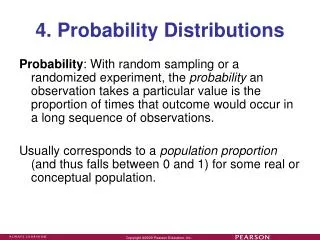
Topic 5: Probability Distributions. Achievement Standard 90646 Solve Probability Distribution Models to solve straightforward problems 4 Credits Externally Assessed NuLake Pages 278 322. NORMAL DISTRIBUTION. PART 2. Lesson 3: Making a continuity correction.

E N D
Topic 5: Probability Distributions Achievement Standard 90646 Solve Probability Distribution Models to solve straightforward problems 4 Credits Externally Assessed NuLake Pages 278 322
NORMAL DISTRIBUTION PART 2
Lesson 3: Making a continuity correction • Go over 1 of the final 2 qs from HW (combined events). NuLake p303. • How to calculate normal distribution probabilities using your Graphics Calculator. To practice using GC: Do Sigma (NEW – photocopy): p358 – Ex. 17.01 (Q3 only). Write qs on board as a quiz. • Continuity corrections – how and when to make them. Work: Fill in handout on cont. corr., then NuLake p309: Q42-46. Finish for HW. *Don’t do Q47.
Using your Graphics Calc. for Standard Normal problems • MENU, STAT, DIST,NORM; then there are three options:* Npd – you will not have to use this option* Ncd – for calculating probabilities* InvN – for inverse problems • NB: On your graphics calculator shaded areas are from -∞ to the point. • To enter -∞ you type – EXP 99. • To enter +∞ you type EXP 99.
Using your Graphics Calc. for Standard Normal problems • MENU, STAT, DIST,NORM; then there are three options:* Npd – you will not have to use this option* Ncd – for calculating probabilities* InvN – for inverse problems • NB: On your graphics calculator shaded areas are from -∞ to the point. • To enter -∞ you type – EXP 99. • To enter +∞ you type EXP 99. E.g. 1: If m=178, s=5, P(175X 184) = ? MENU, STAT, DIST, NORM, Ncd lower: 175, upper: 184, σ: 5, μ: 178
Using your Graphics Calc. for Standard Normal problems • MENU, STAT, DIST,NORM; then there are three options:* Npd – you will not have to use this option* Ncd – for calculating probabilities* InvN – for inverse problems • NB: On your graphics calculator shaded areas are from -∞ to the point. • To enter -∞ you type – EXP 99. • To enter +∞ you type EXP 99. E.g. 1: If m=178, s=5, P(175X 184) = 0.61067 MENU, STAT, DIST, NORM, Ncd lower: 175, upper: 184, σ: 5, μ: 178
MENU, STAT, DIST,NORM; then there are three options:* Npd – you will not have to use this option* Ncd – for calculating probabilities* InvN – for inverse problems • NB: On your graphics calculator shaded areas are from -∞ to the point. • To enter -∞ you type – EXP 99. • To enter +∞ you type EXP 99. E.g.1: If m=178, s=5, P(175X 184) = 0.61067 MENU, STAT, DIST, NORM, Ncd lower: 175, upper: 184, σ: 5, μ: 178 E.g.2: If m=30, s=3.5, P(X 31) = ? MENU, STAT, DIST, NORM, Ncd lower: -EXP99, upper: 31, σ: 3.5, μ: 30
MENU, STAT, DIST,NORM; then there are three options:* Npd – you will not have to use this option* Ncd – for calculating probabilities* InvN – for inverse problems • NB: On your graphics calculator shaded areas are from -∞ to the point. • To enter -∞ you type – EXP 99. • To enter +∞ you type EXP 99. E.g.1: If m=178, s=5, P(175X 184) = 0.61067 MENU, STAT, DIST, NORM, Ncd lower: 175, upper: 184, σ: 5, μ: 178 E.g.2: If m=30, s=3.5, P(X 31) = 0.61245 MENU, STAT, DIST, NORM, Ncd lower: -EXP99, upper: 31, σ: 3.5, μ: 30
10 minutes • Do Sigma (NEW) p358. • Ex. 17.01 • Q3 on the board as a quiz. • MENU, STAT, DIST,NORM; then there are three options:* Npd – you will not have to use this option* Ncd – for calculating probabilities* InvN – for inverse problems • NB: On your graphics calculator shaded areas are from -∞ to the point. • To enter -∞ you type – EXP 99. • To enter +∞ you type EXP 99. E.g.1: If m=178, s=5, P(175X 184) = 0.61067 MENU, STAT, DIST, NORM, Ncd lower: 175, upper: 184, σ: 5, μ: 178 E.g.2: If m=30, s=3.5, P(X 31) = 0.61245 MENU, STAT, DIST, NORM, Ncd lower: -EXP99, upper: 31, σ: 3.5, μ: 30
Making a Continuity Correction (USE THE HANDOUT)
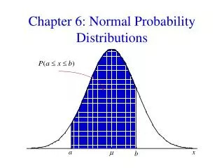
Heights of Year 13 males in NZ are normally distributed with mean 174 cm and standard deviation 6 cm. If they are measured to the nearest cm, calculate the probability that the height of a student is more than 165 cm. 17.02A 165 174 165 174 164.5 165 165.5 Actual curve for heights of students(continuous) Distribution when rounding heights (discrete histogram) For example the probability that a student was 165 cm tall would have to be represented by a column with base 164.5 to 165.5
Heights of Year 13 males in NZ are normally distributed with mean 174 cm and standard deviation 6 cm. If they are measured to the nearest cm, calculate the probability that the height of a student is more than 165 cm. 165 174 165 174 164.5 164.5 165 165 165.5 165.5 Actual curve for heights of students(continuous) Distribution when rounding heights (discrete histogram) For example the probability that a student was 165 cm tall would have to be represented by a column with base 164.5 to 165.5
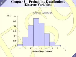
Heights of Year 13 males in NZ are normally distributed with mean 174 cm and standard deviation 6 cm. If they are measured to the nearest cm, calculate the probability that the height of a student is more than 165 cm. 165 174 165 174 164.5 164.5 165 165 165.5 165.5 Actual curve for heights of students(continuous) Distribution when rounding heights (discrete histogram) For example the probability that a student was 165 cm tall would have to be represented by a column with base 164.5 to 165.5 because any student with a height in thisintervalwould be recorded as having a height of165 cm.
Heights of Year 13 males in NZ are normally distributed with mean 174 cm and standard deviation 6 cm. If they are measured to the nearest cm, calculate the probability that the height of a student is more than 165 cm. 165 174 165 174 164.5 164.5 165 165 165.5 165.5 To find the cut-off point for continuity corrections, move up or down to the midpoint between two whole-numbers. In this example the wording is ‘more than 165’, so move up to 165.5. P(X > 165) = P(X > ?) with continuity correction.
Heights of Year 13 males in NZ are normally distributed with mean 174 cm and standard deviation 6 cm. If they are measured to the nearest cm, calculate the probability that the height of a student is more than 165 cm. 165 174 165 174 164.5 164.5 165 165 165.5 165.5 To find the cut-off point for continuity corrections, move up or down to the midpoint between two whole-numbers. In this example the wording is ‘more than 165’, so move up to 165.5. P(X > 165)≈P(X > 165.5) with continuity correction. ≈0.9217 (4 sf)
Continuity Correction If we use a Normal Distribution to approximate a variable that is DISCRETE, we must make a Continuity Correction.
Continuity Correction If we use a Normal Distribution to approximate a variable that is DISCRETE, we must make a Continuity Correction.
Continuity Correction If we use a Normal Distribution to approximate a variable that is DISCRETE, we must make a Continuity Correction.
Continuity Correction If we use a Normal Distribution to approximate a variable that is DISCRETE, we must make a Continuity Correction.
Continuity Correction If we use a Normal Distribution to approximate a variable that is DISCRETE, we must make a Continuity Correction.
Continuity Correction If we use a Normal Distribution to approximate a variable that is DISCRETE, we must make a Continuity Correction.
Continuity Correction If we use a Normal Distribution to approximate a variable that is DISCRETE, we must make a Continuity Correction.
Continuity Correction Do NuLake qs on “Continuity Corrections for a Normal Distribution”: Pg. 311-313: Q4246 (NOTE: Don’t do Q47). If we use a Normal Distribution to approximate a variable that is DISCRETE, we must make a Continuity Correction.
Continuity Correction Do NuLake qs on “Continuity Corrections for a Normal Distribution”: Pg. 311-313: Q4246 (NOTE: Don’t do Q47). If we use a Normal Distribution to approximate a variable that is DISCRETE, we must make a Continuity Correction.
Continuity Correction Do NuLake qs on “Continuity Corrections for a Normal Distribution”: Pg. 311-313: Q4246 (NOTE: Don’t do Q47). If we use a Normal Distribution to approximate a variable that is DISCRETE, we must make a Continuity Correction.
Continuity Correction Do NuLake qs on “Continuity Corrections for a Normal Distribution”: Pg. 311-313: Q4246 (NOTE: Don’t do Q47). If we use a Normal Distribution to approximate a variable that is DISCRETE, we must make a Continuity Correction.
Lesson 4: Inverse normal problems where you are given the probability and asked to calculate the x-value. Learning outcome: Calculate the x cut-off score based on given probabilities, and a given mean and SD. Work: • Inverse calculations using standard normal. • Inverse calculations – standardising Examples • Do Sigma (new - photocopy): p366 – Ex. 17.03.
Inverse questions - the other way around Where you’re told the probability and have to find the z-values. Examples: (a) Find the value of z giving the area of 0.3770 between 0 and z. z = ?
P(0 < Z <z) = 0.377 What isz? Answer (from tables): z = ?
P(0 < Z <z) = 0.377 What isz? Answer (from tables): z= 1.16
Inverse questions - the other way around Where you’re told the probability and have to find the z-values. Examples: (a) Find the value of z giving the area of 0.3770 between 0 and z. z = 1.16
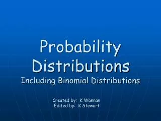
Inverse questions - the other way around Where you’re told the probability and have to find the z-values. Examples: (a) Find the value of z giving the area of 0.3770 between 0 and z. z = 1.16 • Find the value of z if the area • to the right of z is only 0.05. z = ?
P(0 < Z <z) = 0.45 What isz? Answer (from tables): z = ?
P(0 < Z <z) = 0.45 What isz? Answer (from tables): z = 1.645
Inverse questions - the other way around Where you’re told the probability and have to find the z-values. Examples: (a) Find the value of z giving the area of 0.3770 between 0 and z. z = 1.16 • Find the value of z if the area • to the right of z is only 0.05. z = 1.645
Inverse problems where you’re given the probability, m and s, and asked to find the value of X. x= + z z= x–m s can be re-arranged to solve for x E.g. A normally distributed random variable has a mean of 24 & std. deviation of 4.7. What value has only 5% of the distribution above it? i.e. P(X> xcut-off) = 0.05. We’re told that m =24 and s =4.7. What is the value, xcut-off?
z= x–m s can be re-arranged to solve for x x= + z E.g. A normally distributed random variable has a mean of 24 & std. deviation of 4.7. What value has only 5% of the distribution above it? i.e. P(X> xcut-off) = 0.05. We’re told that m =24 and s =4.7. What is the value, xcut-off?
z= x–m s can be re-arranged to solve for x x= + z E.g. A normally distributed random variable has a mean of 24 & std. deviation of 4.7. What value has only 5% of the distribution above it? i.e. P(X> xcut-off ) = 0.05. We’re told that m =24 and s =4.7. What is the value, xcut-off ?
z= x–m s can be re-arranged to solve for x x= + z E.g. A normally distributed random variable has a mean of 24 & std. deviation of 4.7. What value has only 5% of the distribution above it? i.e. P(X> xcut-off ) = 0.05. We’re told that m =24 and s =4.7. What is the value, xcut-off ? First do using working (standardise it), then check with G.Calc. s= 4.7 First find the z cut-off like in the last example m= 24 xcut-off = ?
P(0 < Z <z) = 0.45 What isz? Answer (from tables): z = ?
P(0 < Z <z) = 0.45 What isz? Answer (from tables): z = 1.645
z= x–m s can be re-arranged to solve for x x= + z E.g. A normally distributed random variable has a mean of 24 & std. deviation of 4.7. What value has only 5% of the distribution above it? i.e. P(X> xcut-off ) = 0.05. We’re told that m =24 and s =4.7. What is the value, xcut-off ? First do using working (standardise it), then check with G.Calc. zcut-off =1.645 m= 24 xcut-off = ?
z= x–m s can be re-arranged to solve for x x= + z E.g. A normally distributed random variable has a mean of 24 & std. deviation of 4.7. What value has only 5% of the distribution above it? i.e. P(X> xcut-off ) = 0.05. We’re told that m =24 and s =4.7. What is the value, xcut-off ? First do using working (standardise it), then check with G.Calc. zcut-off =1.645 m= 24 xcut-off =
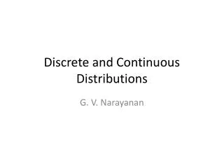
z= x–m s can be re-arranged to solve for x x= + z E.g. A normally distributed random variable has a mean of 24 & std. deviation of 4.7. What value has only 5% of the distribution above it? i.e. P(X> xcut-off ) = 0.05. We’re told that m =24 and s =4.7. What is the value, xcut-off ? First do using working (standardise it), then check with G.Calc. STAT, DIST, NORM, InvN Area: _____ , σ: 4.7, μ: 24 zcut-off =1.645 m= 24 xcut-off = Area: Enter total area to the LEFT of xcut-off.
z= x–m s can be re-arranged to solve for x x= + z E.g. A normally distributed random variable has a mean of 24 & std. deviation of 4.7. What value has only 5% of the distribution above it? i.e. P(X> xcut-off ) = 0.05. We’re told that m =24 and s =4.7. What is the value, xcut-off ? First do using working (standardise it), then check with G.Calc. STAT, DIST, NORM, InvN Area: 1-0.05 , σ: 4.7, μ: 24 zcut-off =1.645 m= 24 xcut-off = Area: Enter total area to the LEFT of xcut-off.
z= x–m s can be re-arranged to solve for x x= + z E.g. A normally distributed random variable has a mean of 24 & std. deviation of 4.7. What value has only 5% of the distribution above it? i.e. P(X> xcut-off ) = 0.05. We’re told that m =24 and s =4.7. What is the value, xcut-off ? First do using working (standardise it), then check with G.Calc. STAT, DIST, NORM, InvN Area: 1-0.05 , σ: 4.7, μ: 24 = ____ zcut-off =1.645 m= 24 xcut-off = Area: Enter total area to the LEFT of xcut-off.
z= x–m s can be re-arranged to solve for x x= + z E.g. A normally distributed random variable has a mean of 24 & std. deviation of 4.7. What value has only 5% of the distribution above it? i.e. P(X> xcut-off ) = 0.05. We’re told that m =24 and s =4.7. What is the value, xcut-off ? First do using working (standardise it), then check with G.Calc. STAT, DIST, NORM, InvN Area: 1-0.05 , σ: 4.7, μ: 24 = 0.95 zcut-off =1.645 m= 24 xcut-off = Area: Enter total area to the LEFT of xcut-off.
z= x–m s can be re-arranged to solve for x x= + z Once you’ve copied down the e.g. & working: Do Sigma (NEW version): p366 – Ex. 17.03 Complete for HW. Extension (after you’ve finished this): NuLake p307 & 308 E.g. A normally distributed random variable has a mean of 24 & std. deviation of 4.7. What value has only 5% of the distribution above it? i.e. P(X> xcut-off ) = 0.05. We’re told that m =24 and s =4.7. What is the value, xcut-off ? First do using working (standardise it), then check with G.Calc. STAT, DIST, NORM, InvN Area: 1-0.05 , σ: 4.7, μ: 24 = 0.95 zcut-off =1.645 m= 24 xcut-off = 31.73 Area: Enter total area to the LEFT of xcut-off.
Lesson 5: Inverse normal problems where you must calculate the mean or SD • Calculate the mean if given the SD and the probability of X taking a certain domain of values. • Calculate the SD if given the mean and the probability of X taking a certain domain of values. Sigma (new - PHOTOCOPY): p369, Ex 17.04.
STARTER: Question from what we did last lesson: Inverse Normal: Calculating the x cut-off score.