Discrete and Continuous Distributions
Discrete and Continuous Distributions. G. V. Narayanan. Discrete Probability Distributions. Bernoulli Probability Function Binomial Probability Function HyperGeometric Probability Function Poisson Probability Function. Continuous Probability Distributions. Uniform Probability Function

Discrete and Continuous Distributions
E N D
Presentation Transcript
Discrete and Continuous Distributions G. V. Narayanan
Discrete Probability Distributions • Bernoulli Probability Function • Binomial Probability Function • HyperGeometric Probability Function • Poisson Probability Function
Continuous Probability Distributions • Uniform Probability Function • Normal Probability Function • Standard Normal Probability Function • LogNormal Probability Function • Exponential Probability Function • Geometric Probability Function • Weibull Probability Function
Understand Random Variable • A Random variable is a NUMERIC VALUE assigned to a ‘quantity’ or ‘property to an Object or item’ • Examples of QUANTITY: Quantity can be an ‘item’ or ‘property of any object’ or ‘length’ or ‘width’ or ‘thickness’ or ‘Area’ or ‘Answers to a Questionaire’ or ‘any scientific numeric values’ • Random Variable ‘Value’ can be either ‘DISCRETE’ or ‘Continuous Interval’ • Mostly, a Random Variable is represented by symbol ‘X’ (Upper case Letter, never Lower case letter) • Mostly, a Random Variable ‘Value’ is represented by symbol ‘x’ (Lower case letter, never Upper case letter)
Random Variable Values of a distribution • Examples of Random Variable Values: • ‘Discrete’ Random Variable Values for the toss of a COIN: Head or Tail => Assigned Values are ‘0’ (zero) for Tail (or Head) or ‘1’ (one) for Head (or Tail) • ‘Discrete’ Random Variable Values for the roll of a Dice: Face up 1, Face up 2, Face up 3, Face up 4, Face up 5, Face up 6 => Assigned Values are ‘1’ (one) for Face up 1 etc • Discrete Random Variable Values for the number of New cars sold is any positive number, 0,1,2,3, … • Discrete Random Variable Values for the number of students is an positive number less than Max Value
Random Variable Values of a distribution • Examples of Random Variable Values: • ‘Continuous’ Random Variable Values for the height of students in a university: Any Positive Real valued number in an interval, say between (3 feet and 7 feet) with a decimal or in feet and inches • ‘Continuous’ Random Variable Values for the impurities in a liquid in units of parts per millions: any Positive real values number in an interval, say between 3 and 10 PPM • ‘Continuous’ Random Variable Values for the Length or Diameter of Rods: any positive real values between 0 and maximum value
About Population Parameters Each Probability Distribution has either ONE or TWO or Three population parameters
The Population Parameters of a Distribution • We always talk about Either ‘Population’ Or ‘Sample’ Data from measurements or from ‘Population’ Data • We will ALWAYS discuss: 1) ‘Probability’ ‘Mass’ or ‘Density’ ‘Distribution’ Functions; 2) ‘Cumulative’ Probability Distributions; 3) ‘Inverse’ Cumulative Probability Distributions For a GIVEN set of ‘Population’ Parameters These population parameters are NOT the SAME for ALL Distributions
The Population Parameters of a Distribution • For Bernoulli Distribution, the probability of ‘success’ or ‘failure’ or ‘defective’ etc is the ONLY population parameter, denoted by symbol ‘p’ • For Binomial Distribution, the TWO population parameters are: N (Total data count) and ‘p’ of Random Variable at a value • For Poisson Distribution, the only population parameter is denoted by symbol ‘lamda’, this lamda equals ‘N*p’ for approximating Binomial distribution for N > 20 and p < 0.05 • Note: Text treats Poisson as Discrete Distribution where as Poisson can be used for Continuous Random Variable in an interval
The Population Parameters of a Distribution • HyperGeometric Distribution has THREE parameter: N( Total Data count), n (Sample Data count) and k (number of successes within ‘n’ selected samples of N items) • The Normal Distribution has TWO population parameters: Mean value ‘mu’ and std deviation ‘sigma’. • For Standard Normal Distribution, Mean = 0 and Stddev = 1
The Population Parameters of a Distribution • LogNormal Distribution has Two Parameters: Mean and StdDev • Exponential Distribution has One Parameter • Weibull Distribution has Two Parameters, Alpha and Beta
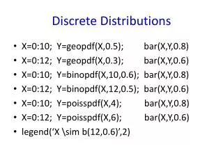
Discrete RV Probability Distributions Binomial Distribution Hypergeometric Distribution Poisson Distribution Geometric Distribution
Bernoulli Distribution Function • Bernoulli Trials are independent (assumed) p(success) = p p(Failure)=1-p • Random Variable X ~ Bernoulli(p) • Probability Mass Function of X is: p(1) = P(X=1) = p p(0) = P(X=0) = 1-p [Random Variable Values are Discrete Values ‘0’ and ‘1’] • Mean = p • Variance = p*(1-p)
Binomial Distribution Function • Binomial Distribution (Sum of Bernoulli Trials): • Bernoulli Trials are independent (assumed) p(success) = p p(Failure)=1-p • Binomial Random Variable X ~ Binomial(n, p) • Probability Mass Function of X is: p(x) = P(X=x) = for x = 0,1,2… [Random Variable Values are Discrete Integer Values of x ] • Mean = n*p • Variance = n*p*(1-p)
Geometric Distribution Function • Binomial Distribution (Sum of Bernoulli Trials): • Bernoulli Trials are independent (assumed) p(success) = p p(Failure)=1-p • Binomial Random Variable X ~ Geometric(p) • (X represents the number of trials upto including first success • Probability Mass Function of X is: p(x) = P(X=x) = for x = 1,2… [Random Variable Values are Discrete Integer Values of x ] • Mean = • Variance =
Hypergeometric Distribution Function • Hypergeometric Distribution (Sum of Bernoulli Trials): • Hypergeometric Random Variable X~Hypergeom(N,k,n) • Probability Mass Function of X is: p(x) = P(X=x) = for max(0, k+n –N) ≤ x ≤ min(n,k) [Random Variable Values are Discrete Integer Values of x ] • Mean = • Variance = n*
Poisson Distribution Function • Poisson Distribution (can approximate Binomial Distribution): • Poisson Random Variable X ~ Poisson(λ) • Probability Mass Function of X is: p(x) = P(X=x) = for positive integer x value [Random Variable Values are Discrete Integer Values of x ] • Mean = λ (approximate n*p for n < 20 and p < 0.05) • Variance = λ
Computing Probability of Binomial Distribution • See Text Page 206 Example 4.7 • Find P(X=5) for Bin(10,0.4) • Here n=10 and p = 0.4 • P(X=5) = • Hence, P(X=5) = 0.2007 • Check against Minitab
Computing Probability of Hypergeometric Distribution • See Text Page 232 Example 4.28 • Find P(X=3) for hypergeom(50,12,10) • Here N=50, k=12, n=10 • P(X=3) = • Hence, P(X=3) = 0.2703 • Check against Minitab
Computing Probability of Poisson Distribution • See Text Page 221 Example 4.21 • Find P(X=17) for Poisson(5*3) • Here (lamda) λ= 5*3 (mean hits in 3 sec) • P(X=17) = • Hence, P(X=17) = 0.0847 • Check against Minitab
Continuous RV Probability Distributions Uniform Distribution Standard Normal Distribution Normal Distribution LogNormal Distribution Exponential Distribution Weibull Distribution
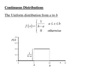
Uniform Distribution Function • UNIFORM Distribution: • Bernoulli Trials are independent (assumed) within an interval(a,b) with Uniform probability density value given two parameters • Uniform Random Variable X ~ Uniform(μ,) • Probability Density Function of X is: p(x) = f(x) = for any value between a < x < b, otherwise 0 [Random Variable Values are Continuous values in an interval of x between x=a and x=b ] Cumulative Probability P(X < x) = • Mean = • Variance =
Standard Normal Distribution Function • STANDARD NORMAL Distribution (also called Standard GAUSSIAN Distribution): • Bernoulli Trials are independent (assumed) within an interval(-∞,∞) with Standard NORMAL probability density value given two parameters μ=0 and σ = 1 • Standard Normal Random Variable Z ~ Normal(0,1) • Probability Density Function of Z is: p(z) = f(z) = for any value between -∞ < z < ∞ [Random Variable Values are Continuous values in an interval of z between z=-∞ and z=∞ ] Cumulative Probability P(Z < z) = • Mean = 0 • Variance = 1
Normal Distribution Function • NORMAL Distribution (also called GAUSSIAN Distribution): • Bernoulli Trials are independent (assumed) within an interval(-∞,∞) with NORMAL probability density value given two parameters • Normal Random Variable X ~ Normal(μ,) • Probability Density Function of X is: p(x) = f(x) = for any value between -∞ < x < ∞ [Random Variable Values are Continuous values in an interval of x between x=-∞ and x=∞ ] Cumulative Probability P(X < x) = • Mean = μ • Variance =
LogNormal Distribution Function • LogNORMAL Distribution (Related to Normal Distribution): • Bernoulli Trials are independent (assumed) within an interval(-∞,∞) with LogNORMAL probability density value given two parameters • LogNormal Random Variable Y ~ Normal(μ,) where X=log(Y) • Random Variable Y = • Probability Density Function of X is: p(x) = f(x) = for any value between -∞ < x < ∞ [Random Variable Values are Continuous values in an interval of x between x=-∞ and x=∞ ] Cumulative Probability P(X < x) = • Mean = μ • Variance =
Exponential Distribution Function • Exponential Distribution (one parameter): • Exponential Random Variable X ~ Exp(λ) • Probability Density Function of X is: p(x) = f(x) = for positive x > 0 value, = zero for x < 0 Random Variable Values are continuous Values of x • Mean = • Variance =
Weibull Distribution Function • WEIBULL Distribution (Two parameters): • Weibull Random Variable X ~ Weibull(α,β) • Probability Density Function of X is: p(x) = f(x) = for positive x > 0, = zero for x < 0 Random Variable Values are continuous Values of x • Mean = • Variance =
Computing Probability of Uniform Distribution • See Text Page 272 Example 4.63 • Find P(10<X<15) for Uniform(0,30) • Here a=0 and b=30 • P(10<X<15) = P(X <15) – P(X <10) • Hence, P(10<X<15) = • Check against Minitab
Computing Probability of Standard Normal Distribution • See Text Page 244 Example 4.41 • Find P(X < 0.47) for StdNormal(0,1) • Here μ=0 and σ = 1 • P(X<0.47) = = 0.6808 (Lookup Table) • See Text Page 244 Example 4.42 • Find P(X > 1.38) for StdNormal(0,1) • Here μ=0 and σ = 1 • P(X>1.38) = 1 - = 1-0.9162 (Lookup Table) • P(X>1.38) = 0.0838 • Check against Minitab
Computing Probability of Normal Distribution • See Text Page 246 Example 4.47 • Find P(2.49 < X < 2.51) for Normal(2.505,0.008sq) • Here μ=2.505 and σ = 0.008 • P(2.49<X<2.51) = P(X < 2.51) – P(X < 2.49) • P(2.49<X<2.51) = - = • Convert x=2.49 and x=2.51 to z-score (standard Normal value); z is -1.88 for x=2.49 and z is 0.63 for x=2.51 • P(-1.88<X<0.63) = - = • Hence, P(2.49<X<2.51) = P(-1.88<z<0.63) = 0.7357-0.0301 • =0.7056; 70.56% meet specification • Check against Minitab
Computing Probability of LogNormal Distribution • See Text Page 258 Example 4.53 • Find P( Y > 4 days) using Normal(1,0.5sq) • Here μ=1 and σ = 0.5; Here we use ln(Y) as normal distribution • P(Y>4) = P(ln(y)> ln(4)) = P(ln(Y) > 1.386) • P(ln(Y) > 1.386 ) = 1 - • Convert x=1.386 to z-score (standard Normal value); z is 0.77 for x=1.386 • P(ln(Y)>1.386) = P(X > 1.386) = 1 - = 0.2206 • Check against Minitab
Computing Probability of Exponential Distribution • See Text Page 264 Example 4.58 • Find P(T > 5) for T ~ Exponential(0.25) • Here λ = 0.25 • P(T > 5) = 1 – P(T ≤ 5) = 1 – (1 - • Hence, P(T > 5) = 0.2865 • Check against Minitab
Compute Uncertainity of Probability Distribution Mean and Variance If Population parameters are unknown, compute uncetainity on parameters computed using SAMPLE data.
Sample Data Values of Population Parameters • If Population parameters are UNKNOWN, then Sample Data is used to compute Equivalent Population Parameters, • For Example, if Mean of Population is UNKNOWN, the mean of Sample (s) can be used as equivalent to Mean of Population (Mu) • Same reasoning goes for Standard Deviation value • StdDev of Sample Data can be used as StdDev value of a population. • The UNCERTANITY of error due to using Sample for obtaining Population parameters must be COMPUTED
Computing Uncertainty of Mean and Standard Deviation for a Binomial Distribution • Sample mean is p-hat = = • Error in computing Mean of population: Unbiased • Uncertainty error in p-hat is: • Variance in p-hat = (p*(1-p))/n • See Text page 210 summary
Normal Probability Plot • Read Section 4.10
Central Limit Theorem • Read section 4.11 • Very Important section in Statstics • See Page 290 BLUE BOX Statements • Jist • X-bar ( Sample Mean) ~ Normal(μ,/n) • Sum of sample observations ~ Normal(nμ,n) • (Read symbol ‘~’ as ‘behave as’)
MiniTab Use in Computing Probability for Binomial Distribution • Use Menu • CalcProbabilityDistributionsBinomial
MiniTab Use in Computing Probability for Poisson Distribution • Use Menu • CalcProbabilityDistributionsPoisson
MiniTab Use in Computing Probability for Hypergeometric Distribution • Use Menu • CalcProbabilityDistributionsHypergeometric • See text • Page 232
MiniTab Use in Computing Probability for Standard Normal Distribution • Use Menu • CalcProbabilityDistributionsNormal
Minitab use to compute Inverse Cumulative Probability for Standard Normal Distribution Distribution • CalcProbability Distributions Normal