Download

1 / 52
530 likes | 752 Vues
Discrete Probability Distributions (Random Variables and Discrete Probability Distributions). Chapter 5 BA 201. Random Variables. Random Variables. A random variable is a numerical description of the outcome of an experiment. A discrete random variable may assume either a

E N D
Discrete Probability Distributions(Random Variables andDiscrete Probability Distributions) Chapter 5 BA 201
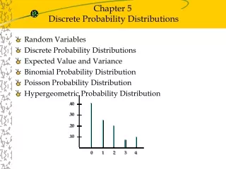
Random Variables A random variable is a numerical description of the outcome of an experiment. A discrete random variable may assume either a finite number of values or an infinite sequence of values. Example: 1, 2, 3, … A continuous random variable may assume any numerical value in an interval or collection of intervals. Example: 1.0, 1.1, 1.2, …
Discrete Random Variable with a Finite Number of Values JSL Appliances Let x = number of TVs sold at the store in one day, where x can take on 5 values (0, 1, 2, 3, 4) We can count the TVs sold, and there is a finite upper limit on the number that might be sold (which is the number of TVs in stock).
Discrete Random Variable with an Infinite Sequence of Values JSL Appliances Let x = number of customers arriving in one day, where x can take on the values 0, 1, 2, . . . We can count the customers arriving, but there is no finite upper limit on the number that might arrive.
Random Variables Type Question Random Variable x Family size x = Number of dependents reported on tax return Discrete Continuous x = Distance in miles from home to the store site Distance from home to store Own dog or cat Discrete x = 1 if own no pet; = 2 if own dog(s) only; = 3 if own cat(s) only; = 4 if own dog(s) and cat(s)
Discrete Probability Distributions The probability distribution for a random variable describes how probabilities are distributed over the values of the random variable. We can describe a discrete probability distribution with a table, graph, or formula.
Discrete Probability Distributions The probability distribution is defined by a probability function, denoted by f(x), which provides the probability for each value of the random variable. The required conditions for a discrete probability function are: f(x) > 0 f(x) = 1
Discrete Probability Distributions JSL Appliances 80/200
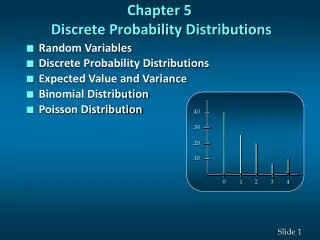
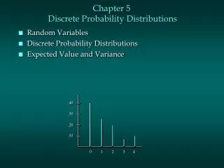
.50 .40 .30 .20 .10 Discrete Probability Distributions JSL Appliances Graphical representation of probability distribution Probability 0 1 2 3 4 Values of Random Variable x (TV sales)
Expected Value The expected value, or mean, of a random variable is a measure of its central location. E(x) = = x f(x) The expected value is a weighted average of the values the random variable may assume. The weights are the probabilities. The expected value does not have to be a value the random variable can assume.
Variance and Standard Deviation The variance summarizes the variability in the values of a random variable. Var(x) = 2 = (x - )2f(x) The variance is a weighted average of the squared deviations of a random variable from its mean. The weights are the probabilities. The standard deviation, , is defined as the positive square root of the variance.
Expected Value JSL Appliances 0 * 0.40 expected number of TVs sold in a day
Variance JSL Appliances Standard deviation of daily sales = = 1.2884 TVs
Discrete Uniform Probability Distribution The discrete uniform probability distribution is the simplest example of a discrete probability distribution given by a formula. The discrete uniform probability function is f(x) = 1/n the values of the random variable are equally likely where: n = the number of values the random variable may assume
Scenario A non-profit sends donation solicitations with pre-printed amounts. Based on past years, the non-profit knows approximately how many people will donate each amount. Compute the expected value of x, variance, and standard deviation.
Binomial Probability Distribution • Four Properties of a Binomial Experiment • 1. The experiment consists of a sequence of n • identical trials. • 2. Two outcomes, success and failure, are possible • on each trial. 3. The probability of a success, denoted by p, does not change from trial to trial. stationarity assumption 4. The trials are independent.
Binomial Probability Distribution Our interest is in the number of successes occurring in the n trials. We let x denote the number of successes occurring in the n trials.
Binomial Probability Distribution • Binomial Probability Function where: x = the number of successes p = the probability of a success on one trial n = the number of trials f(x) = the probability of x successes in n trials
Binomial Probability Distribution • Binomial Probability Function Probability of a particular sequence of trial outcomes with x successes in n trials Number of experimental outcomes providing exactly x successes in n trials
Binomial Probability Distribution Evans Electronics Evans Electronics is concerned about a low retention rate for its employees. In recent years, management has seen a turnover of 10% of the hourly employees annually. Thus, for any hourly employee chosen at random, management estimates a probability of 0.1 that the person will not be with the company next year. Choosing 3 hourly employees at random, what is the probability that 1 of them will leave the company this year?
Binomial Probability Distribution Evans Electronics The probability of the first employee leaving and the second and third employees staying, denoted (S, F, F), is given by p(1 – p)(1 – p) With a 0.10 probability of an employee leaving on any one trial, the probability of an employee leaving on the first trial and not on the second and third trials is given by (0.10)(0.90)(0.90) = (0.10)(0.90)2= 0.081
Binomial Probability Distribution Evans Electronics Two other experimental outcomes also result in one success and two failures. The probabilities for all three experimental outcomes involving one success follow. Probability of Experimental Outcome p(1 – p)(1 – p) = (0.1)(0.9)(0.9) = 0.081 (1 – p)p(1 – p) = (0.9)(0.1)(0.9) = 0.081 (1 – p)(1 – p)p = (0.9)(0.9)(0.1) = 0.081 Total = 0.243 Experimental Outcome (S, F, F) (F, S, F) (F, F, S)
Binomial Probability Distribution Using a tree diagram Evans Electronics x 1st Worker 2nd Worker 3rd Worker Prob. L (0.1) 0.0010 3 L (0.1) 0.0090 2 S (0.9) L (0.1) 0.0090 L (0.1) 2 S (0.9) 1 0.0810 S (0.9) L (0.1) 2 0.0090 L (0.1) 1 0.0810 S (0.9) S (0.9) L (0.1) 1 0.0810 S (0.9) 0 0.7290 S (0.9)
Binomial Probability Distribution Evans Electronics Using the probability function Let: p = 0.10, n = 3, x = 1
Binomial Probability Distribution • Expected Value E(x) = = np • Variance • Var(x) = 2 = np(1 -p) • Standard Deviation
Binomial Probability Distribution Evans Electronics • Expected Value E(x) = np= 3(.1) = 0.3 employees out of 3 • Variance Var(x) = np(1 – p) = 3(0.1)(0.9) = 0.27 • Standard Deviation
Scenario Kearn Manufacturing (KM) submits bids for sales a number of times each month. Based on an analysis of past bids, the sales director knows that on average 34% of bids result in sales. KM Last week the sales director submitted three bids. The sales director would like to know how likely it is that two of the bids will result in sales. What are n, x (that two bids result in sales), and p. What is f(x)? Draw a tree diagram illustrating this scenario. Compute the expected value of x. Compute the variance and standard deviation.
Poisson Probability Distribution A Poisson distributed random variable is often useful in estimating the number of occurrences over a specified interval of time or space It is a discrete random variable that may assume an infinite sequence of values (x = 0, 1, 2, . . . ).
Poisson Probability Distribution Examples of a Poisson distributed random variable: the number of knotholes in 14 linear feet of pine board the number of vehicles arriving at a toll booth in one hour Bell Labs used the Poisson distribution to model the arrival of phone calls.
Poisson Probability Distribution • Two Properties of a Poisson Experiment • The probability of an occurrence is the same • for any two intervals of equal length. • The occurrence or nonoccurrence in any • interval is independent of the occurrence or • nonoccurrence in any other interval.
Poisson Probability Distribution • Poisson Probability Function where: x = the number of occurrences in an interval f(x) = the probability of x occurrences in an interval = mean number of occurrences in an interval e = 2.71828
Poisson Probability Distribution • Poisson Probability Function • Since there is no stated upper limit for the number • of occurrences, the probability function f(x) is • applicable for values x = 0, 1, 2, … without limit. • In practical applications, x will eventually become • large enough so that f(x) is approximately zero and • the probability of any larger values of x becomes • negligible.
Poisson Probability Distribution Mercy Hospital Patients arrive at the emergency room of Mercy Hospital at the average rate of 6 per hour on weekend evenings. What is the probability of 4 arrivals in 30 minutes on a weekend evening?
Poisson Probability Distribution Using the probability function Mercy Hospital = 6/hour = 3/half-hour, x = 4 Note: Example:
Poisson Probabilities 0.25 0.20 0.15 Probability 0.10 0.05 0.00 1 2 3 4 5 6 7 8 9 10 0 Number of Arrivals in 30 Minutes Poisson Probability Distribution Mercy Hospital actually, the sequence continues: 11, 12, …
Poisson Probability Distribution • A property of the Poisson distribution is that • the mean and variance are equal. m = s 2
Poisson Probability Distribution Mercy Hospital Variance for Number of Arrivals During 30-Minute Periods m = s2 = 3
Scenario On weekdays between 11:00 a.m. and 2:00 p.m., Joe’s Pizza receives approximately one order every two minutes. What is the expected number of orders per hour? What is the probability three orders will arrive in a five-minute period? What is the probability no orders will arrive in a five-minute period? What is the variance of the number of orders arriving?
Discrete Probability Distributions • x takes discrete values. • Values for f(x) may be subjectively assigned, assigned based on frequency of occurrence, or uniform. • If f(x) is uniform, f(x) = 1/n where n is the number of values x may assume. E(x) = μ = [x * f(x)] Var(x) = 2 = [(x – μ)2 * f(x)]
Binomial Probability Distributions • Four properties: (1) n identical trials, (2) success or failure, (3) p does not change, and (4) trials are independent. • x is the number of successes. E(x) = μ = n * p Var(x) = 2 = n * p * (1-p)