Download
1 / 37
390 likes | 582 Vues
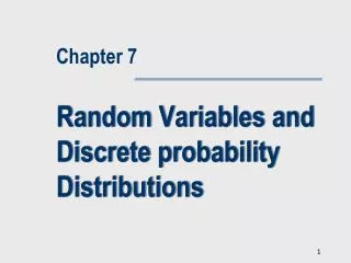
Random Variables and Discrete probability Distributions. Chapter 7. 7.1 Random Variables and Discrete Probability Distribution. Many times simple events in the sample space can be assigned numerical values. A random variable can then be defined that takes on these values.

E N D
Random Variables and Discrete probability Distributions Chapter 7
7.1 Random Variables and Discrete Probability Distribution • Many times simple events in the sample space can be assigned numerical values. A random variable can then be defined that takes on these values. • The random variable reflects a certain characteristic of interest of the experimental outcome. • Examples: • The number of cars entering a gas station in the next five minutes. • The amount of gas filled in a gas tank by a driver. • The grade in a physics test. • The number of new employees to be hired next month.
7.1 Random Variables and Discrete Probability Distribution • There are two types of random variables: • Discrete random variable • Continuous random variable. • A random variable is discrete if it can assume only a countable number of values. • A random variable is continuous if it can assume an uncountable number of values.
0 1 2 3 ... A short demonstration:Discrete and Continuous Random Variables Discrete random variable Continuous random variable Only certain values can be assigned to the random variable Any value within the range where the variable is defined can be selected 0 Therefore, the number of values is countable Therefore, the number of values is uncountable
Discrete Probability Distribution • A table, formula, or graph that lists all possible values a discrete random variable can assume, together with the probabilities associated with each value, is called a discrete probability distribution. • To calculate the probability that the random variable X assumes the value x, P(X = a), • add the probabilities of all the simple events for which X is equal to ‘a’, or • Use probability calculation tools (such as tree diagram),
Simple event x Probability TT 0 1/4 HT 1 1/4 TH 1 1/4 HH 2 1/4 x p(x) 0 1/4 1 1/2 2 1/4 H HH (½)(½)=1/4 H (½)(½)=1/4 HT T H TH (½)(½)=1/4 T T (½)(½)=1/4 TT Discrete Probability Distribution • Example 1 • Find the probability distribution of the random variable describing the number of heads that turn-up when a coin is flipped twice. • Solution
Requirements for a Discrete Distribution • If a random variable can assume values xi, then the following must be true: • With the probability distribution we can more conveniently calculate probabilities (see example 2) next.
Distribution and Relative Frequencies • Example 2 • A survey reveals the following frequencies for the number of colored TV per household. Number of TVs Number of Households x p(x)0 1,218 0 1218/Total = .012 1 32,379 1 32379/Total = .319 2 37,961 2 .374 3 19,387 3 .191 4 7,714 4 .076 5 2,842 5 .028Total 101,5011.000
Determining Probability of Events Example 2 – continued Calculate the probability of the following events: • P(The number of colored TVs is 3) = P(X=3) =.191 • P(The number of colored TVs is two or more) = P(X³2)=P(X=2)+P(X=3)+P(X=4)+P(X=5)= .319+.374+…= .669
Determining the Probability Distribution and the Probability of Events • Example 3 • The number of cars a dealer is selling daily were recorded in the last 100 days. This data was summarized as follows: • Estimate the probability distribution. • State the probability of selling more than 2 cars a day. Daily sales Frequency 0 5 1 15 2 35 3 25 4 20 100
.35 .25 .20 .15 .05 • The probability of selling more than 2 cars a day is P(X>2) = P(X=3) + P(X=4) = .25 + .20 = .45 Determining the Probability Distribution and the Probability of Events • Example 3 - Solution From the table of frequencies we can calculate the relative frequencies, which becomes our estimated probability distribution Daily sales Relative Frequency 0 5/100=.05 1 15/100=.15 2 35/100=.35 3 25/100=.25 4 20/100=.20 1.00 X 0 1 2 3 4
Developing a Probability Distribution • Example 4 • A mutual fund sales person knows that there is 20% chance of closing a sale on each call she makes. • What is the probability distribution of the number of sales if she plans to call three customers? • Solution • Let us use probability rules and probability tree • Define event Ai = {a sale is made in the iit phone call}.
Developing a Probability Distribution • Assuming each phone call is independent of all other phone calls, we can assign the following probabilities to each branch on the tree: (.2)(.2)(.8)= .032 A1 and A2 and A3 A1 and A2 and A3C A1 and A2C and A3 A1c and A2 and A3 A1 and A1C andA3C A1C andA2 and A3C A1C and A2C andA3 A1C andA2C andAC • X P(x) • .23 = .008 • 3(.032)=.096 • 3(.128)=.384 • 0 .83 = .512 If X represents the number of sales made, then.. (click) (.2)(.8)(.8)= .128
Expected value and Variance Describing the PopulationProbability Distribution
The Expected Value (Mean) • Given a discrete random variable X with values xi, that occurs with probabilities p(xi), the population mean of X is.
The Population Variance • Let X be a discrete random variable with possible values xi that occur with probabilities p(xi), and let E(xi) = m. The variance of X is defined by
The Mean and the Variance • Example 5 Find the mean the variance and the standard deviation for the population of the number of colored TV per household in example 2 • Solution • E(X) = m = Sxip(xi) = 0p(0)+1p(1)+2p(2)+…= 0(.012)+1(.319)+2(.374)+… = 2.084 • V(X) = s2 = S(xi - m)2p(xi) = (0-2.084)2p(0)+(1-2.084)2p(1) + (2-2.084)2+… =1.107 • s = 1.1071/2 = 1.052 Using a shortcut formula for the variance
The Mean and the Variance • Solution – continued • The variance can also be calculated as follows:
7.4 The Binomial Distribution • The binomial experiment has the following characteristics: • There are n trials (n is finite and fixed). • Each trial can result in one out of two outcomes, success or a failure. • The probability p of a success is the same for all the trials. • All the trials of the experiment are independent.
Binomial Random Variable • The binomial random variable counts the number of successes in n trials of the binomial experiment. • The possible values of this count are 0,1, 2, …,n, and therefore the binomial variable is discrete.
The Binomial Probability Distribution The binomial probability distribution is described bythe following closed form formula:
S2 S1 F2 S2 F1 F2 Developing the Binomial Probability Distribution (n = 3) P(S2|S1) P(F2|S1) P(S1)=p P(F1)=1-p P(S2|F1) P(F2|F1)
S3 P(S3|S2,S1) S2 P(S3)=p S1 P(F3)=1-p F3 P(F3|S2,S1) P(S3|F2,S1) S3 P(S3)=p P(SFS)=p(1-p)p P(F2|S1) P(F2)=1-p P(F3)=1-p F2 P(F3|F2,S1) F3 P(SFF)=p(1-p)2 S3 P(S3|S2,F1) P(FSS)=(1-p)p2 P(S3)=p S2 P(S2)=p P(S2|F1) P(F3)=1-p P(F3|S2,F1) F3 P(FSF)=(1-p)P(1-p) S3 P(S3|F2,F1) P(FFS)=(1-p)2p F1 P(S3)=p P(F2|F1) P(F2)=1-p F2 P(F3)=1-p P(F3|F2,F1) F3 P(FFF)=(1-p)3 Developing the Binomial Probability Distribution (n = 3) P(SSS)=p3 P(S2|S1) P(S2)=p P(SSF)=p2(1-p) P(S1)=p Since the outcome of each trial is independent of the previous outcomes, we can replace the conditional probabilities with the unconditional probabilities. P(F1)=1-p
Developing the Binomial Probability Distribution (n = 3) P(X = 3) = P(Three successes) = P(SSS) = p3 P(X = 2) = P(Two successes, one Failure) = P(SSF) + P(SFS) + P(FSS) = p2(1-p) + p(1-p)p + (1-p)pp = p2(1-p) + p2(1-p) + p2(1-p) = 3 p2(1-p). P(X = 1) = P(One success, two failures) = P(SFF) + P(FSF) + P(FFS) = p(1-p)2 + (1-p)p(1-p) + (1-p)2p = p(1-p)2 + p(1-p)2 + p(1-p)2 = 3 p(1-p)2 P(X = 0) = P(Three failures) = P(FFF) = (1-p)3
Calculating the Binomial Probability • Example 10 • Pat Statsdud takes a course in statistics, and intends to rely on luck to pass the next quiz. • The quiz consists on 10 multiple choice questions with 5 possible choices for each question, only one is the correct answer. • Pat will guess the answer to each question • Find the following probabilities • Pat gets no answer correct • Pat gets two answer correct? • Pat fails the quiz
Calculating the Binomial Probability • Solution • Checking the conditions: • Only one out of two outcomes can occur (An answer can be either correct or incorrect). • There is a fixed finite number of trials (There are 10 questions in the test, n=10). • Each answer is independent of the others. • The probability p of a correct answer does not change from question to question(20% chance that an answer is correct).
Calculating the Binomial Probability • Solution – Continued • Determining the binomial probabilities: Let X = the number of correct answers
This is called cumulative probability Calculating the Binomial Probability • Solution – Continued • Determining the binomial probabilities: Pat fails the test if she gets less than 5 correct answers. P(X£4) = p(0) + p(1) + p(2) + p(3) + p(4) = .1074 + .2684 + .3020 + .2013 + .0881 =.9672
Mean and Variance - Binomial Variable E(X) = m = np V(X) = s2 = np(1-p)
Mean and variance of binomial variable • Example 11 • If all the students in Pat’s class practice the same learning behavior like she does, what is the mean and the standard deviation of the quiz mark? • Solution • m = np = 10(.2) = 2. • s = [np(1-p)]1/2 = [10(.2)(.8)]1/2 = 1.26.
Binomial Distribution - summary • Example 12 • Records show that 30% of the customers in a shoe store make their payments using a credit card. • This morning 20 customers purchased shoes. • Use the binomial table to answer some questions stated in the next few slides.
Binomial Distribution - summary • Solution • First we verify that this is a binomial experiment: • There are two possible outcomes of which only one will take place (paid with the credit card or not) • There is a finite number of trials (20 customers are observed) • Customers pay independently • Each customer has the same probability to pay with a credit card (. 30).
p k n = 20 .995 Binomial Distribution - summary • Solution – continued • Find the probability that at most 11 customers use a credit card. In what follows we demonstrate the usage of the Binomial Table .01……….. .30 0 . . 11 P(X £ 11) = .995
Binomial Distribution - summary • To calculate P(X £ 11) when p = 0.3 and n = 20, type in an empty cell the following:=binomdist(11,20,0.3,1). Then click outside the cell. • To calculate P(X = 11) type the following: =binomdist(11,20,0.3,0) • To calculate P(X ³ 11) type the following:= 1 - binomdist(10,20,0.3,1) In what follows we demonstrate how to use Excel to determine binomial probabilities
p k Binomial Distribution - summary • What is the probability that at least 3 but not more than 6 customers used a credit card? At least 3 butnot more than 6 Not more than 6 .01……….. .30 0 2 . 6 P(3£X£6)= P(X=3 or 4 or 5 or 6) = .035 Click P(X£6) - P(X£2) .573 .608 =.608 - .035 = .573 3 4 5 6 0 1 2 3 4 5 6
Binomial Distribution - summary • Find the probability that exactly 14 customers did not use a credit card. Let Y be the number of customers who did not use a credit card, while X (as before) the number of those who did use a credit card.P(Y=14) = P(X=6) = P(X £ 6) - P(X £ 5) = .608 - .416 = .192 • Using Excel to solve the last two questions: • P(3 £ X £ 6) = binomdist(6,20,0.3,1) – binomdist(2,20,0.3,1) • P(Y = 14) = binomdist(14,20,0.7,0)
Binomial Distribution - summary • What is the expected number of customers who used a credit card? E(X) = np = 20(.30) = 6