Chapter 5 Discrete Random Variables and Probability Distributions
EF 507 QUANTITATIVE METHODS FOR ECONOMICS AND FINANCE FALL 2008. Chapter 5 Discrete Random Variables and Probability Distributions. Introduction to Probability Distributions. Random Variable Represents a possible numerical value from a random experiment. Random Variables. Ch. 5. Ch. 6.

Chapter 5 Discrete Random Variables and Probability Distributions
E N D
Presentation Transcript
EF 507 QUANTITATIVE METHODS FOR ECONOMICS AND FINANCE FALL 2008 Chapter 5 Discrete Random Variables and Probability Distributions
Introduction to Probability Distributions • Random Variable • Represents a possible numerical value from a random experiment Random Variables Ch. 5 Ch. 6 Discrete Random Variable Continuous Random Variable
Discrete Random Variables • Can only take on a countable number of values Examples: • Roll a die twice Let X be the number of times 4 comes up (then X could be 0, 1, or 2 times) • Toss a coin 5 times. Let X be the number of heads (then X = 0, 1, 2, 3, 4, or 5)
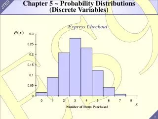
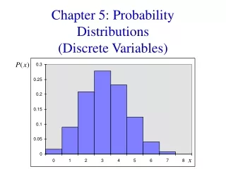
Discrete Probability Distribution Experiment: Toss 2 Coins. Let X = # heads. x ValueProbability 0 1/4 = 0.25 1 2/4 = 0.50 2 1/4 = 0.25 Show P(x) , i.e., P(X = x) , for all values of x: 4 possible outcomes Probability Distribution T T T H H T 0.50 0.25 Probability H H 0 1 2 x
Probability DistributionRequired Properties • P(x) 0 for any value of x • The individual probabilities sum to 1; (The notation indicates summation over all possible x values)
Cumulative Probability Function • The cumulative probability function, denoted F(x0), shows the probability that X is less than or equal to x0 • In other words,
Expected Value • Expected Value (or mean) of a discrete distribution (Weighted Average) • Example: Toss 2 coins, x = # of heads, compute expected value of x: E(x) = (0 x 0.25) + (1 x 0.50) + (2 x 0.25) = 1.0 x P(x) 0 0.25 1 0.50 2 0.25
Variance and Standard Deviation • Variance of a discrete random variable X • Standard Deviation of a discrete random variable X
Standard Deviation Example • Example: Toss 2 coins, X = # heads, compute standard deviation (recall E(x) = 1) Possible number of heads = 0, 1, or 2
Functions of Random Variables • If P(x) is the probability function of a discrete random variable X , and g(X) is some function of X ,then the expected value of function g is
Linear Functions of Random Variables • Let a and b be any constants. • a) i.e., if a random variable always takes the value a, it will have mean a and variance 0 • b) i.e., the expected value of b·X is b·E(x)
Linear Functions of Random Variables (continued) • Let random variable X have mean µx and variance σ2x • Let a and b be any constants. • Let Y = a + bX • Then the mean and variance of Y are • so that the standard deviation of Y is
Probability Distributions Probability Distributions Ch. 5 Discrete Probability Distributions Continuous Probability Distributions Ch. 6 Binomial Uniform Hypergeometric Normal Poisson Exponential
The Binomial Distribution Probability Distributions Discrete Probability Distributions Binomial Hypergeometric Poisson
Bernoulli Distribution • Consider only two outcomes: “success” or “failure” • Let P denote the probability of success (1) • Let 1 – P be the probability of failure (0) • Define random variable X: x = 1 if success, x = 0 if failure • Then the Bernoulli probability function is
Bernoulli DistributionMean and Variance • The mean is µ = P • The variance is σ2 = P(1 – P)
Sequences of x Successes in n Trials • The number of sequences with x successes in nindependent trials is: Where n! = n·(n – 1)·(n – 2)· . . . ·1 and 0! = 1 • These sequences are mutually exclusive, since no two can occur at the same time
Binomial Probability Distribution 1-A fixed number of observations, n • e.g., 15 tosses of a coin; ten light bulbs taken from a warehouse 2-Two mutually exclusive and collectively exhaustive categories • e.g., head or tail in each toss of a coin; defective or not defective light bulb • Generally called “success” and “failure” • Probability of success is P , probability of failure is 1 – P 3-Constant probability for each observation • e.g., Probability of getting a tail is the same each time we toss the coin 4-Observations are independent • The outcome of one observation does not affect the outcome of the other
Possible Binomial Distribution Settings • A manufacturing plant labels items as either defective or acceptable • A firm bidding for contracts will either get a contract or not • A marketing research firm receives survey responses of “Yes I will buy” or “No I will not” • New job applicants either accept the offer or reject it
Binomial Distribution Formula n ! - X X n P(x) = P (1- P) ) x ! ( - ! n x P(x) = probability of x successes in n trials, with probability of success Pon each trial x = number of ‘successes’ in sample, (x = 0, 1, 2, ..., n) n = sample size (number of trials or observations) P = probability of “success” Example: Flip a coin four times, let x = # heads: n = 4 P = 0.5 1 - P = (1 - 0.5) = 0.5 x = 0, 1, 2, 3, 4
Example: Calculating a Binomial Probability What is the probability of one success in five observations if the probability of success is 0.1? x = 1, n = 5, and P = 0.1
Binomial Distribution • The shape of the binomial distribution depends on the values of P and n Mean n = 5 P = 0.1 P(x) .6 • Here, n = 5 and P = 0.1 .4 .2 0 x 0 1 2 3 4 5 n = 5 P = 0.5 P(x) .6 • Here, n = 5 and P = 0.5 .4 .2 x 0 0 1 2 3 4 5
Binomial DistributionMean and Variance • Mean • Variance and Standard Deviation Where n = sample size P = probability of success (1 – P) = probability of failure
Binomial Characteristics Examples n = 5 P = 0.1 P(x) Mean .6 .4 .2 0 x 0 1 2 3 4 5 n = 5 P = 0.5 P(x) .6 .4 .2 x 0 0 1 2 3 4 5
Using Binomial Tables (Table 2, p.844) Examples: n = 10, x = 3, P = 0.35: P(x = 3|n =10, p = 0.35) = 0.2522 n = 10, x = 8, P = 0.45: P(x = 8|n =10, p = 0.45) = 0.0229
Using PHStat • Select PHStat / Probability & Prob. Distributions / Binomial…
Using PHStat (continued) • Enter desired values in dialog box Here: n = 10 p = .35 Output for x = 0 to x = 10 will be generated by PHStat Optional check boxes for additional output
PHStat Output P(x = 3 | n = 10, P = .35) = .2522 P(x > 5 | n = 10, P = .35) = .0949
The Hypergeometric Distribution Probability Distributions Discrete Probability Distributions Binomial Hypergeometric Poisson
The Hypergeometric Distribution • “n” trials in a sample taken from a finite population of size N • Sample taken without replacement • Outcomes of trials are dependent • Concerned with finding the probability of “X” successes in the sample where there are “S” successes in the population
Hypergeometric Distribution Formula Where N = population size S = number of successes in the population N – S = number of failures in the population n = sample size x = number of successes in the sample n – x = number of failures in the sample
Using the Hypergeometric Distribution • Example: 3 different computers are checked from 10 in the department. 4 of the 10 computers have illegal software loaded. What is the probability that 2 of the 3 selected computers have illegal software loaded? N = 10n = 3 S = 4x = 2 The probability that 2 of the 3 selected computers have illegal software loaded is 0.30, or 30%.
Hypergeometric Distribution in PHStat • Select: PHStat / Probability & Prob. Distributions / Hypergeometric …
Hypergeometric Distribution in PHStat (continued) • Complete dialog box entries and get output … • N = 10 n = 3 • S = 4 x = 2 P(X = 2) = 0.3
The Poisson Distribution Probability Distributions Discrete Probability Distributions Binomial Hypergeometric Poisson
The Poisson Distribution • Apply the Poisson Distribution when: 1-You wish to count the number of times an event occurs in a given continuous interval 2-The probability that an event occurs in one subinterval is very small and is the same for all subintervals 3-The number of events that occur in one subinterval is independent of the number of events that occur in the other subintervals 4-There can be no more than one occurrence in each subinterval 5-The average number of events per unit is (lambda)
Poisson Distribution Formula where: x = number of successes per unit = expected number of successes per unit e = base of the natural logarithm system (2.71828...)
Poisson Distribution Characteristics • Mean • Variance and Standard Deviation where = expected number of successes per unit
Using Poisson Tables (Table 5, p.853) Example: Find P(X = 2) if = 0.50
Example 1: The average number of trucks arriving on any one day at a truck depot in a certain city is known to be 12. What is the probability that on a given day fewer than nine trucks will arrive at this depot? • X: number of trucks arriving on a given day. • Lambda=12 • P(X<9) = SUM[p(x;12)] from 0 to 8 = 0.1550 • Example 2: The number of complaints that a call center receives per day is a random variable having a Poisson distribution with lambda=3.3. Find the probability that the call center will receive only two complaints on any given day.
Graph of Poisson Probabilities Graphically: = 0.50 P(X = 2) = 0.0758
Poisson Distribution Shape • The shape of the Poisson Distribution depends on the parameter : = 0.50 = 3.00
Poisson Distribution in PHStat • Select: PHStat / Probability & Prob. Distributions / Poisson…
Poisson Distribution in PHStat (continued) • Complete dialog box entries and get output … P(X = 2) = 0.0758
Joint Probability Functions • A joint probability function is used to express the probability that X takes the specific value x and simultaneouslyY takes the value y, as a function of x and y • The marginal probabilities are
Conditional Probability Functions • The conditional probability function of the random variable Y expresses the probability that Y takes the value y when the value x is specified for X. • Similarly, the conditional probability function of X, given Y = y is:
Independence • The jointly distributed random variables X and Y are said to be independentif and only if their joint probability function is the product of their marginal probability functions: for all possible pairs of values x and y • A set of k random variables are independent if and only if
Covariance • Let X and Y be discrete random variables with means μX and μY • The expected value of (X - μX)(Y - μY) is called the covariancebetween X and Y • For discrete random variables • An equivalent expression is
Covariance and Independence • The covariance measures the strength of the linear relationship between two variables • If two random variables are statistically independent, the covariance between them is 0 • The converse is not necessarily true Example: mean_x=0; mean_y= -1/3; E(xy)=0; sigma_xy=0 So the covariance is 0, but for x=-1 and y=-1 f(x,y) is not equal to g(x)h(y)