Random Variables and Probability Distributions
Random Variables and Probability Distributions. Kanchala sudtachat. Content. Random Variables Probability Discrete Random Variables Discrete Uniform Distribution Binomial Distribution Poisson Distribution Continuous Random Variables Continuous Uniform Distribution Normal Distribution


Random Variables and Probability Distributions
E N D
Presentation Transcript
Random Variables and Probability Distributions Kanchalasudtachat
Content • Random Variables • Probability • Discrete Random Variables • Discrete Uniform Distribution • Binomial Distribution • Poisson Distribution • Continuous Random Variables • Continuous Uniform Distribution • Normal Distribution • t- Distribution • Exponential Distribution • Normal Approximation to the Binomial and Poisson Distributions • Normal Probability Plots
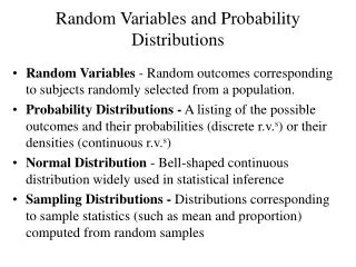
Random Variables • A measurement is usually denoted by a variable such as X. • A variable whose measured value can change. (random variable) Discrete Random Variable – a finite set of real numbers Continuous Random Variable – an interval of real numbers
Probability • A random variable is used to describe a measurement. • Probability is used to quantify the likelihood, that a measurement falls within some set of values. “The chance that X, the length of a manufactured part, is between 10.8 and 11.2 millimeters is 25%” • Probability • Degree of belief • A relative frequency (or proportion) of repeated replicates that fall in the interval will be percent, uses a long run proportion.
Probability Properties • Given a set E, the set of real number is denoted as R. • Each element is in one and only one of the sets E1, E2,…,Ek. • Applying Probability Properties • Ex: X denotes the life in hours of standard fluorescent tubes • P(X ≤ 5000) = 0.1, P(5000<X≤ 6000) = 0.3, P(X> 8000) = 0.4
Discrete Random Variables • Example 3-19 A voice communication network for a business contains 48 external lines. At a particular time, the system is observed and some of the lines are being used. • Example 3-20 The analysis of the surface of a semiconductor wafer records the number of particles of contamination that exceed a certain size. Define the random variable X to equal the number of particles of contamination.
Probability Mass Function (pmf) • The probability distribution of a random variable X is a description of the probabilities associated with the possible values of X. • It is convenient to express the probability in terms of a formula. Example 3-21 There is a chance that a bit transmitted through a digital transmission channel is received in error. Let X equal the number of bits in error in the next 4 bits transmitted. The possible value for X are {0, 1, 2, 3, 4}
Probability Mass Function (pmf) Cumulative Distribution Function (cdf)
Cumulative Distribution Function (cdf) • Example 3-22 In previous example, the probability mass function for X • P(X=0) = 0.6561 P(X=1) = 0.2916 P(X=2) = 0.0486 • P(X=3) = 0.0036P(X=4) = 0.0001
Mean and Variance Example 3-23 For the number of bits in error in the previous example. Determining µ and σ2
Mean and Variance Example 3-24 Two new product designs are to be compared on the basis for revenue potential. Marketing feels that the revenue from design A can be predicted quite accurately to be $3 million. The revenue potential of design B is more difficult to assess. Marketing concludes that there is a probability of 0.3 that the revenue from design B will be $7 million, but there is a 0.7 probability that the revenue will be only $2 million. Which design would you choose?
Discrete Uniform Distribution Example The first digit of a part’s serial number is equally likely to be any one of the digits 0 through 9. If one part is selected from a large batch and X is the first digit of the serial number.
Discrete Uniform Distribution Example As in previous example 3-19, let the random variable X denote the number of the 48 voice lines that are in use at a particular time. Assume that X is a discrete uniform random variable with a range of 0 to 48. Determining µ and σ2
Binomial Distribution • Each of these random experiments can be thought of as consisting of a series of repeated, random trials. • The random variable in each case is a count of the number of trials that meet a specified criterion.
Binomial Distribution • Example 3-25 In Example 3-21, assume that the chance that a bit transmitted through a digital transmission channel is received in error is 0.1. Also assume that the transmission trials are independent. Let X = the number of bits in error in the next 4 bits transmitted. • Determine P (X=2)
Binomial Distribution • Example 3-27 Each sample of water has a 10% chance of containing high levels of organic solids. Assume that the samples are independent with regard to the presence of the solids. Determine the probability that in the next 18 samples, exactly 2 contain high solids. • Example 3-28 For the number of transmitted bits received in error in Example 3-21, n = 4 and p = 0.1
Poisson Process • Events occur randomly in an interval time. • The number of events over an interval time is a discrete random variable.
Poisson Process • Example 3-30 Flaws occur at random along the length of the thin copper wire. Let X denote the random variable that counts the number of flaws in a length of L millimeters of wire and suppose that the average number of flaws in L millimeters is λ.
Poisson Process • In general, consider an interval T of real number partitioned into subintervals of small length Δt and assume that as Δt tends to zero, • The probability of more than one event in a subinterval tends to zero, • The probability of one event in a subinterval tends to λ Δt /T • The event in each subinterval is independent of other subintervals A random experiment with these properties is called a Poisson Process.
Poisson Process • Example 3-31 For the case of the thin copper wire, suppose that the number of flaws follows a Poisson distribution with a mean of 2.3 flaws per millimeter. Determine the probability of exactly 2 flaws in 1 millimeter of wire.
Poisson Process • Example 3-32 Contamination is a problem in the manufacture of optical storage disks. The number of particles of contamination that occur on an optical disk has a Poisson distribution, and the average number of particles per centimeter squared of media surface is 0.1. The area of a disk under study is 100 squared centimeters. Determine the probability that 12 particles occur in the area of a disk under study.
Continuous Random Variables • Probability density Function f(x) are used to describe physical systems. • Considering the density of a loading on a long, thin beam. For any point x along the beam, the density can be described by a functions (in grams/cm).
Probability density function • A pdf is zero for x values that cannot occur • f(x) is used to calculate an area the represents the probability that X assumes a value in [a, b].
Probability density function • Example 3-2 Let the continuous random variable X denote the current measured in a thin copper wire in mill-amperes. Assume that the range of X is [0, 20 mA], and assume that the probability density function of X is f(x)=0.05 for 0 ≤ x ≤ 20. What is the probability that a current measurement is less than 10 mill-amperes?
Probability density function • Example 3-3 Let the continuous random variable X denote the distance in micrometers from the start of a track on a magnetic disk until the first flaw. Historical data show that the distribution of X can be modeled by a pdf For what proportion of disks is the distance • to the first flaw greater than 1000 micrometers?
Cumulative Distribution Function • Example 3-4 Consider the distance to flaws in Example 3-3 with pdf • f(x) = 1/2000 exp(-x/2000) • For x ≥ 0. Determine the cdf.
Mean and Variance • Example 3-5 For the copper current measurement in Example 3-2, the mean of X is • Example 3-6 For the distance to a flaw in Example 3-3, the mean of X is
Normal Distribution • Histograms have characteristic shape as bell shapes. • The random variable that equals the average result over the replicates tends to have a normal distribution as the number of replicates becomes large.
Normal Distribution • Example 3-7 Assume that the current measurements in a strip of wire follow a normal distribution with a mean of 10 mill-amperes and a variance of 4 mill-amperes2. What is the probability that a measurement exceeds 13 mill-amperes?
Using standard normal random variable • Example 3-8 Assume that Z is a standard normal random variable. Appendix A Table I provides probabilities of the form P(Z ≤ z). The use of Table I to fine P(Z ≤ 1.5).
Example 3-9 • P(Z > 1.26) • P(Z < -0.86) • P(Z > -1.37) • P(Z < 1.37) • P(-1.25 < Z < 0.37) • P(Z ≤ -4.6) • Fine the value z such that P(Z > z) = 0.05 • Find the value of z such that P(-z < Z < z)=0.99
Example 3-10 • Suppose the current measurements in a strip of wire follow a normal distribution with a mean of 10 mill-amperes and a variance of 4 mill-amperes2. What is the probability that a measurement exceeds 13 mill-amperes?
Example 3-11 • Continuing the previous example, what is the probability that a current measurement is between 9 and 11 mill-amperes?
Example 3-12 • In the transmission of a digital signal, assume that the background noise follows a normal distribution with a mean of 0 volt and standard deviation of 0.45 volt. If the system assumes that a digital 1 has been transmitted when the voltage exceeds 0.9, what is the probability of detecting a digital 1 when none was sent?
Example 3-13 • The diameter of a shaft in storage drive is normally distributed with mean 0.2508 inch and standard deviation 0.0005 inch. The specifications on the shaft are 0.2500 ± 0.0015 inch. What proportion of shafts conforms to specifications?
t-Distribution • When is unknown • Small sample size • Degree of freedom (k) = n-1 • Significant level = • t, k
Exponential Distribution • Let the random variable X denote the length from any starting point on the wire until a flaw is detected. • Let the random variable N denote the number of flaws in x mill-meters of wire. Assume that the mean number of flaws is λ per mill-meters.
Example 3-33 • In a large corporate computer network, use log-on to the system can be modeled as a Poisson process with a mean of 25 log-on per hour. What is the probability that there are no log-on in an interval of 6 minutes?