Download

1 / 113
1.2k likes | 1.57k Vues
Continuous Random Variables and Probability Distributions. 4. Probability Density Functions. 4.1. Probability Density Functions.

E N D
Continuous Random Variables and Probability Distributions • 4
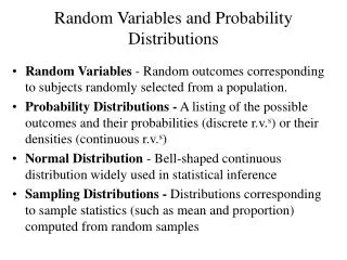
Probability Density Functions • A discrete random variable is one whose possible values either constitute a finite set or else can be listed in an infinite sequence (a list in which there is a first element, a second element, etc.). • A random variable whose set of possible values is an entire interval of numbers is not discrete.
Probability Density Functions • A random variable is continuous if both of the following apply: • 1. Its set of possible values consists either of all numbers in a single interval on the number line or all numbers in a disjoint union of such intervals (e.g., [0, 10] [20, 30]). • 2. No possible value of the variable has positive probability, that is, P(X = c) = 0 for any possible value c.
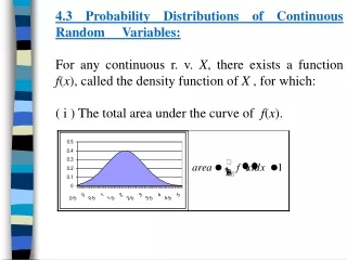
Probability Distributions for Continuous Variables • Definition • Let X be a continuous rv. Then a probability distribution or probability density function (pdf) of X is a function f(x) such that for any two numbers a and b with ab, • P(aXb) =
Probability Distributions for Continuous Variables • That is, the probability that X takes on a value in the interval [a, b] is the area above this interval and under the graph of the density function, as illustrated in Figure 4.2. • The graph of f(x) is often referred to as the density curve. • P(a Xb) = the area under the density curve between a and b • Figure 4.2
Probability Distributions for Continuous Variables • For f(x) to be a legitimate pdf, it must satisfy the following two conditions: • 1. f(x) 0 for all x • 2. = area under the entire graph of f(x) • = 1
Example 4 • The direction of an imperfection with respect to a reference line on a circular object such as a tire, brake rotor, or flywheel is, in general, subject to uncertainty. • Consider the reference line connecting the valve stem on a tire to the center point, and let X be the angle measured clockwise to the location of an imperfection. One possible pdf for X is
Example 4 • cont’d • The pdf is graphed in Figure 4.3. • The pdf and probability from Example 4 • Figure 4.3
Example 4 • cont’d • Clearly f(x) 0. The area under the density curve • is just the area of a rectangle: • (height)(base) = (360) = 1. • The probability that the angle is between 90 and 180 is
Probability Distributions for Continuous Variables • Because whenever 0 ab360 in Example 4.4 and P(aXb) depends only on the width b –a of the interval, X is said to have a uniform distribution. • Definition • A continuous rv X is said to have a uniform distribution on the interval [A, B] if the pdf of X is
Probability Distributions for Continuous Variables • When X is a discrete random variable, each possible value is assigned positive probability. • This is not true of a continuous random variable (that is, the second condition of the definition is satisfied) because the area under a density curve that lies above any single value is zero:
Probability Distributions for Continuous Variables • The fact that P(X = c) = 0 when X is continuous has an important practical consequence: The probability that X lies in some interval between a and b does not depend on whether the lower limit a or the upper limit b is included in the probability calculation: • P(a X b) = P(a < X < b) = P(a < X b) = P(a X < b) • If X is discrete and both a and b are possible values (e.g., X is binomial with n = 20 and a = 5, b = 10), then all four of the probabilities in (4.1) are different. • (4.1)
Example 5 • “Time headway” in traffic flow is the elapsed time between the time that one car finishes passing a fixed point and the instant that the next car begins to pass that point. • Let X = the time headway for two randomly chosen consecutive cars on a freeway during a period of heavy flow. The following pdf of X is essentially the one suggested in “The Statistical Properties of Freeway Traffic” (Transp. Res., vol. 11: 221–228):
Example 5 • cont’d • The graph of f(x) is given in Figure 4.4; there is no density associated with headway times less than .5, and headway density decreases rapidly (exponentially fast) as x increases from .5. • The density curve for time headway in Example 5 • Figure 4.4
Example 5 • cont’d • Clearly, f(x) 0; to show that f(x)dx = 1, we use the calculus result • e–kxdx = (1/k)e–ka. • Then
Example 5 • cont’d • The probability that headway time is at most 5 sec is • P(X 5) = • = .15e–.15(x – .5) dx • =.15e.075 e–15x dx • =
Example 5 • cont’d • = e.075(–e–.75 + e–.075) • = 1.078(–.472 + .928) • = .491 • = P(less than 5 sec) • = P(X < 5)
The Cumulative Distribution Function • The cumulative distribution function (cdf) F(x) for a discrete rv X gives, for any specified number x, the probability P(X x) . • It is obtained by summing the pdf p(y) over all possible values y satisfying y x. • The cdf of a continuous rv gives the same probabilities P(X x) and is obtained by integrating the pdf f(y) between the limits and x.
The Cumulative Distribution Function • Definition • The cumulative distribution function F(x) for a continuous rv X is defined for every number x by • F(x) = P(X x) = • For each x, F(x) is the area under the density curve to the left of x. This is illustrated in Figure 4.5, where F(x) increases smoothly as x increases. • A pdf and associated cdf • Figure 4.5
Example 6 • Let X, the thickness of a certain metal sheet, have a uniform distribution on [A, B]. • The density function is shown in Figure 4.6. • The pdf for a uniform distribution • Figure 4.6
Example 6 • cont’d • For x < A, F(x) = 0, since there is no area under the graph of the density function to the left of such an x. • For x B, F(x) = 1, since all the area is accumulated to the left of such an x. Finally for A x B,
Example 6 • cont’d • The entire cdf is • The graph of this cdf appears in Figure 4.7. • The cdf for a uniform distribution • Figure 4.7
Using F(x) to Compute Probabilities • The importance of the cdf here, just as for discrete rv’s, is that probabilities of various intervals can be computed from a formula for or table of F(x). • Proposition • Let X be a continuous rv with pdf f(x) and cdf F(x). Then for any number a, • P(X > a) = 1 – F(a) • and for any two numbers a and b with a < b, • P(a X b) = F(b) – F(a)
Using F(x) to Compute Probabilities • Figure 4.8 illustrates the second part of this proposition; the desired probability is the shaded area under the density curve between a and b, and it equals the difference between the two shaded cumulative areas. • This is different from what is appropriate for a discrete integer valued random variable (e.g., binomial or Poisson): • P(a X b) = F(b) – F(a – 1) when a and b are integers. • Computing P(a X b) from cumulative probabilities • Figure 4.8
Example 7 • Suppose the pdf of the magnitude X of a dynamic load on a bridge (in newtons) is • For any number x between 0 and 2,
Example 7 • cont’d • Thus • The graphs of f(x) and F(x) are shown in Figure 4.9. • The pdf and cdf for Example 4.7 • Figure 4.9
Example 7 • cont’d • The probability that the load is between 1 and 1.5 is • P(1 X 1.5) = F(1.5) – F(1) • The probability that the load exceeds 1 is • P(X > 1) = 1 – P(X 1) • = 1 – F(1)
Example 7 • cont’d • = 1 – • Once the cdf has been obtained, any probability involving X can easily be calculated without any further integration.
Obtaining f(x) from F(x) • For X discrete, the pmf is obtained from the cdf by taking the difference between two F(x) values. The continuous analog of a difference is a derivative. • The following result is a consequence of the Fundamental Theorem of Calculus. • Proposition • If X is a continuous rv with pdf f(x) and cdf F(x), then at every x at which the derivative F(x) exists, F(x) = f(x).
Example 8 • When X has a uniform distribution, F(x) is differentiable except at x = A and x = B, where the graph of F(x) has sharp corners. • Since F(x) = 0 for x < A and F(x) = 1 for x > B, F(x) = 0 = f(x) for such x. • For A < x < B,
Percentiles of a Continuous Distribution • When we say that an individual’s test score was at the 85th percentile of the population, we mean that 85% of all population scores were below that score and 15% were above. • Similarly, the 40th percentile is the score that exceeds 40% of all scores and is exceeded by 60% of all scores.
Percentiles of a Continuous Distribution • Proposition • Let p be a number between 0 and 1. The (100p)th percentile of the distribution of a continuous rv X, denoted by (p), is defined by • p = F((p)) = f(y) dy • According to Expression (4.2), (p) is that value on the measurement axis such that 100p% of the area under the graph of f(x) lies to the left of (p) and 100(1 – p)% lies to the right. • (4.2)
Percentiles of a Continuous Distribution • Thus (.75), the 75th percentile, is such that the area under the graph of f(x) to the left of (.75) is .75. • Figure 4.10 illustrates the definition. • The (100p)th percentile of a continuous distribution • Figure 4.10
Example 9 • The distribution of the amount of gravel (in tons) sold by a particular construction supply company in a given week is a continuous rv X with pdf • The cdf of sales for any x between 0 and 1 is
Example 9 • cont’d • The graphs of both f(x) and F(x) appear in Figure 4.11. • The pdf and cdf for Example 4.9 • Figure 4.11
Example 9 • cont’d • The (100p)th percentile of this distribution satisfies the equation • that is, • ((p))3 – 3(p) + 2p = 0 • For the 50th percentile, p = .5, and the equation to be solved is 3 – 3 + 1= 0; the solution is = (.5) = .347. If the distribution remains the same from week to week, then in the long run 50% of all weeks will result in sales of less than .347 ton and 50% in more than .347 ton.
Percentiles of a Continuous Distribution • Definition • The median of a continuous distribution, denoted by , is the 50th percentile, so satisfies .5 = F( ) That is, half the area under the density curve is to the left of and half is to the right of . • A continuous distribution whose pdf is symmetric—the graph of the pdf to the left of some point is a mirror image of the graph to the right of that point—has median equal to the point of symmetry, since half the area under the curve lies to either side of this point.
Percentiles of a Continuous Distribution • Figure 4.12 gives several examples. The error in a measurement of a physical quantity is often assumed to have a symmetric distribution. • Medians of symmetric distributions • Figure 4.12
Expected Values • For a discrete random variable X, E(X) was obtained by summing x p(x)over possible X values. • Here we replace summation by integration and the pmf by the pdf to get a continuous weighted average. • Definition • The expected or mean value of a continuous rvX with pdf f(x) is • x= E(X) = x f(x) dy
Example 10 • The pdf of weekly gravel sales X was • (1 – x2) 0 x 1 • 0 otherwise • So • f(x) =
Expected Values • When the pdf f(x) specifies a model for the distribution of values in a numerical population, then is the population mean, which is the most frequently used measure of population location or center. • Often we wish to compute the expected value of some function h(X) of the rv X. • If we think of h(X) as a new rv Y, techniques from mathematical statistics can be used to derive the pdf of Y, and E(Y) can then be computed from the definition.
Expected Values • Fortunately, as in the discrete case, there is an easier way to compute E[h(X)]. • Proposition • If X is a continuous rv with pdf f(x) and h(X) is any function of X, then • E[h(X)] = h(X) = h(x) f (x) dx
Example 11 • Two species are competing in a region for control of a limited amount of a certain resource. • Let X = the proportion of the resource controlled by species 1 and suppose X has pdf • 0 x 1 otherwise • which is a uniform distribution on [0, 1]. (In her book Ecological Diversity, E. C. Pielou calls this the “broken- tick” model for resource allocation, since it is analogous to breaking a stick at a randomly chosen point.) • f(x) =