Understanding Continuous Distributions Through Functions and Graphs
Learn about continuous random variables, probability density functions, uniform, normal, exponential, Weibull, and gamma distributions using functions and graphs.

Understanding Continuous Distributions Through Functions and Graphs
E N D
Presentation Transcript
Continuousrandom variables For a continuous random variable X the probability distribution is described by the probability density function f(x), which has the following properties : • f(x) ≥ 0
Graph: Continuous Random Variableprobability density function, f(x)
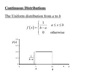
Definition: A random variable , X, is said to have a Uniform distribution from a to b if X is a continuous random variable with probability density function f(x):
The Cumulative Distribution function, F(x)(Uniform Distribution from a to b)
Definition: A random variable , X, is said to have a Normal distribution with mean mand standard deviation sif X is a continuous random variable with probability density function f(x):
Graph: the Normal Distribution(mean m, standard deviation s) s m
Note: Thus the point mis an extremum point of f(x). (In this case a maximum)
Thus the points m – s, m + sare points of inflection of f(x)
Also Proof: To evaluate Make the substitution
Consider evaluating Note: Make the change to polar coordinates (R, q) z = R sin(q) and u = R cos(q)
and Hence or and Using
and or
Consider a continuous random variable, X with the following properties: • P[X ≥0] = 1, and • P[X ≥ a + b] = P[X ≥ a] P[X ≥ b] for all a > 0, b > 0. These two properties are reasonable to assume if X = lifetime of an object that doesn’t age. The second property implies:
The property: models the non-aging property i.e. Given the object has lived to age a, the probability that is lives a further b units is the same as if it was born at age a.
Let F(x) = P[X ≤ x] and G(x) = P[X ≥ x] . Since X is a continuous RV then G(x) = 1 – F(x) (P[X ≥ x] = 0 for all x.) The two properties can be written in terms of G(x): • G(0) = 1, and • G(a + b) = G(a) G(b) for all a > 0, b > 0. We can show that the only continuous function, G(x), that satisfies 1. and 2. is a exponential function
From property 2 we can conclude Using induction Hence putting a = 1. Also putting a = 1/n. Finally putting a = 1/m.
Since G(x) is continuous for all x ≥ 0. If G(1) = 0 then G(x) = 0 for all x > 0 and G(0) = 0 if G is continuous. (a contradiction) If G(1) = 1 then G(x) = 1 for all x > 0 and G() = 1 if G is continuous. (a contradiction) Thus G(1) ≠ 0, 1 and 0 < G(1) < 1 Let l = - ln(G(1)) then G(1) = e-l
To find the density of X we use: A continuous random variable with this density function is said to have the exponential distribution with parameter l.
Graphs of f(x) and F(x) f(x) F(x)
Another derivation of the Exponential distribution Consider a continuous random variable, X with the following properties: • P[X ≥0] = 1, and • P[x ≤ X ≤ x + dx|X ≥ x] = ldx • for all x > 0 and small dx. These two properties are reasonable to assume if X = lifetime of an object that doesn’t age. The second property implies that if the object has lived up to time x, the chance that it dies in the small interval x to x + dx depends only on the length of that interval, dx, and not on its age x.
Determination of the distribution of X Let F (x ) = P[X ≤ x] = the cumulative distribution function of the random variable, X . Then P[X ≥0] = 1 implies that F(0) = 0. Also P[x ≤ X ≤ x + dx|X ≥ x] = ldx implies
for the unknown F. We can now solve the differential equation
Now using the fact that F(0) = 0. This shows that X has an exponential distribution with parameter l.
The Weibull distribution A model for the lifetime of objects that do age.
P[X ≥0] = 1, and • P[x ≤ X ≤ x + dx|X ≥ x] = ldx • for all x > 0 and small dx. Recall the properties of continuous random variable, X, that lead to the Exponential distribution. namely Suppose that the second property is replaced by: • P[x ≤ X ≤ x + dx|X ≥ x] = l(x)dx = axb – 1dx • for all x > 0 and small dx. The second property now implies that object does age. If it has lived up to time x, the chance that it dies in the small interval x to x + dx depends both on the length of that interval, dx, and its age x.
Derivation of the Weibulll distribution A continuous random variable, X satisfies the following properties: • P[X ≥0] = 1, and • P[x ≤ X ≤ x + dx|X ≥ x] = axb-1dx • for all x > 0 and small dx.
Let F (x ) = P[X ≤ x] = the cumulative distribution function of the random variable, X . Then P[X ≥0] = 1 implies that F(0) = 0. Also P[x ≤ X ≤ x + dx|X ≥ x] = axb -1dx implies
for the unknown F. We can now solve the differential equation
again F(0) = 0 implies c = 0. The distribution of X is called the Weibull distribution with parameters a andb.
The Weibull density, f(x) (a= 0.9, b= 2) (a= 0.7, b= 2) (a= 0.5, b= 2)
The Gamma distribution An important family of distibutions
The Gamma Function, G(x) An important function in mathematics The Gamma function is defined for x ≥ 0 by
Properties of Gamma Function, G(x) • G(1) = 1 • G(x + 1) = xG(x) We will use integration by parts to evaluate
Graph: The Gamma Function G(x) x
The Gamma distribution Let the continuous random variable X have density function: Then X is said to have a Gamma distribution with parameters aand l.
Graph: The gamma distribution (a = 2,l = 0.9) (a = 2,l = 0.6) (a = 3,l = 0.6)
Comments • The set of gamma distributions is a family of distributions (parameterized by a and l). • Contained within this family are other distributions • The Exponential distribution – in this case a = 1, the gamma distribution becomes the exponential distribution with parameter l. The exponential distribution arises if we are measuring the lifetime, X, of an object that does not age. It is also used a distribution for waiting times between events occurring uniformly in time. • The Chi-square distribution – in the case a= n/2 and l= ½, the gamma distribution becomes the chi- square (c2) distribution with n degrees of freedom. Later we will see that sum of squares of independent standard normal variates have a chi-square distribution, degrees of freedom = the number of independent terms in the sum of squares.
The Exponential distribution The Chi-square (c2) distribution with n d.f.
Graph: The c2 distribution (n = 4) (n = 5) (n = 6)
Summary Important continuous distributions