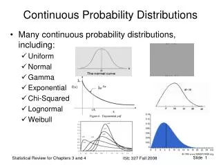
Continuous Probability Distributions
Continuous Probability Distributions. Chapter 8. 0. 1/3. 1/2. 1. 2/3. 8.1 Continuous Probability Distributions.


Continuous Probability Distributions
E N D
Presentation Transcript
Continuous Probability Distributions Chapter 8
0 1/3 1/2 1 2/3 8.1 Continuous Probability Distributions • Unlike a discrete random variable which we studied in Chapter 7, a continuous random variable(連續型隨機變數)is one that can assume an uncountable number of values in the interval (a,b). • We cannot list the possible values because there is an infinite number of them. • Because there is an infinite number of values, the probability that a continuous variable X will assume any particular value is 0. Why? The probability of each value 1/4 + 1/4 + 1/4 + 1/4 = 1 1/3 + 1/3 + 1/3 = 1 1/2 + 1/2 = 1
0 1/3 1/2 1 2/3 8.1 Continuous Probability Distributions As the number of values increases the probability of each value decreases. This is so because the sum of all the probabilities remains 1. When the number of values approaches infinity (because X is continuous) the probability of each value approaches 0. The probability of each value 1/4 + 1/4 + 1/4 + 1/4 = 1 1/3 + 1/3 + 1/3 = 1 1/2 + 1/2 = 1
Point Probabilities are Zero • Because there is an infinite number of values, the probability of each individual value is virtually 0. • Thus, we can determine the probability of a range of values only. • E.g. with a discrete random variable like tossing a die, it is meaningful to talk about P(X=5), say. • In a continuous setting (e.g. with time as a random variable), the probability the random variable of interest, say task length, takes exactly 5 minutes is infinitesimally small, hence P(X=5) = 0. • It is meaningful to talk about P(X ≤ 5).
Area = 1 x1 x2 P(x1≤X≤x2) Probability Density Function • To calculate probabilities we define a probability density function f(x). • A function f(x) is called a probability density function(機率密度函數)(over the range a ≤ x ≤ b if it meets the following requirements: 1) f(x) ≥ 0 for all x between a and b, and 2) The total areaunder the curve between a and b is 1.0 • The probability that X falls between x1 and x2 is found by calculating the area under the graph of f(x) between x1 and x2.
Uniform Distribution(均等分配) • Consider the uniform probability distribution (sometimes called the rectangular probability distribution(矩形分配)). • It is described by the function: f(x) a b x
Uniform Distribution • A random variable X is said to be uniformly distributed if its density function is • The expected value and the variance are
Example 8.1 • The amount of gasoline sold daily at a service station is uniformly distributed with a minimum of 2,000 gallons and a maximum of 5,000 gallons. Find the probability that sales are: • Between 2,500 and 3,000 gallons • More than 4,000 gallons • Exactly 2,500 gallons
Example 8.1 • The daily sale of gasoline is uniformly distributed between 2,000 and 5,000 gallons. • Find the probability that sales are between 2,500 and 3,000 gallons. f(x) = 1/(5000-2000) = 1/3000 for x: [2000,5000] P(2500£X£3000) = (3000-2500)(1/3000) = .1667 There is about a 17% chance that between 2,500 and 3,000 gallons of gas will be sold on a given day. 1/3000 x 2000 2500 3000 5000
Example 8.1 • The daily sale of gasoline is uniformly distributed between 2,000 and 5,000 gallons. • Find the probability that sales are more than 4,000 gallons. f(x) = 1/(5000-2000) = 1/3000 for x: [2000,5000] There is a 33% chance the gas station will sell more than 4,000 gallons on any given day. P(X³4000) = (5000-4000)(1/3000) = .333 1/3000 x 2000 4000 5000
Example 8.1 • The daily sale of gasoline is uniformly distributed between 2,000 and 5,000 gallons. • Find the probability that sales are exactly 2,500 gallons. f(x) = 1/(5000-2000) = 1/3000 for x: [2000,5000] The probability that the gas station will sell exactly 2,500 gallons is zero. P(X=2500) = (2500-2500)(1/3000) = 0 1/3000 x 2000 2500 5000
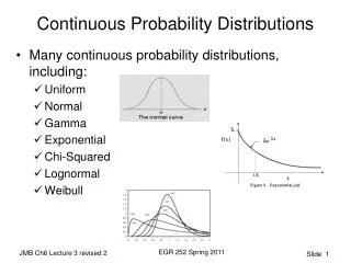
8.2 Normal Distribution(常態分配) • This is the most important continuous distribution. • Many distributions can be approximated by a normal distribution. • The normal distribution is the cornerstone distribution of statistical inference.
Normal Distribution • A random variable X with mean m and variance s2is normally distributed if its probability density function is given by Unlike the range of the uniform distribution (a ≤ x ≤ b), Normal distributions range from minus infinity to plus infinity.
The Normal Distribution • Important things to note: The normal distribution is fully defined by two parameters: its standard deviation andmean The normal distribution is bell shaped and symmetrical about the mean.
The Shape of the Normal Distribution The normal distribution is bell shaped, and symmetrical around m. m 90 110 Why symmetrical? Let m = 100. Suppose x = 110. Now suppose x = 90
The effects of m and s How does the standard deviation affect the shape of f(x)? s= 2 Increasing the standard deviation “flattens” the curve. s =3 s =4 How does the expected value affect the location of f(x)? m = 10 m = 11 m = 12 Increasing the mean shifts the curve to the right.
0 1 1 Standard Normal Distribution • A normal distribution whose mean is 0 and standard deviation is 1 is called the standard normal distribution(標準常態分配). • As we shall see shortly, any normal distribution can be converted to a standard normal distribution with simple algebra. This makes calculations much easier.
Finding Normal Probabilities • Two facts help calculate normal probabilities: • The normal distribution is symmetrical. • Any normal distribution can be transformed into a specific normal distribution called “STANDARD NORMAL DISTRIBUTION” • Example The amount of time it takes to assemble a computer is normally distributed, with a mean of 50 minutes and a standard deviation of 10 minutes. What is the probability that a computer is assembled in a time between 45 and 60 minutes?
Finding Normal Probabilities • Solution • If Xdenotes the assembly time of a computer, we seek the probability P(45<X<60). • This probability can be calculated by creating a new normal variable the standard normal variable. This shifts the mean of X to zero… Every normal variable with some m and s, can be transformed into this Z. Therefore, once probabilities for Z are calculated, probabilities of any normal variable can be found. E(Z) = m = 0, V(Z) = s2 = 1 This changes the shape of the curve…
Finding Normal Probabilities • Example - continued - m 45 - 50 X 60 - 50 P(45<X<60) = P( < < ) s 10 10 = P(-0.5 < Z < 1) To complete the calculation we need to compute the probability under the standard normal distribution
P(0<Z<z0) Using the Standard Normal Table Standard normal probabilities have been calculated and are provided in a table . The tabulated probabilities correspond to the area between Z=0 and some Z = z0 >0 Z = z0 Z = 0
- m 45 - 50 X 60 - 50 P(45<X<60) = P( < < ) s 10 10 z0 = 1 z0 = -.5 Finding Normal Probabilities • Example - continued = P(-.5 < Z < 1) We need to find the shaded area
- m 45 - 50 X 60 - 50 P(45<X<60) = P( < < ) s 10 10 z0 = 1 z0 =-.5 Finding Normal Probabilities • Example - continued = P(-.5<Z<1) = P(-.5<Z<0)+ P(0<Z<1) P(0<Z<1 .3413 z=0
Finding Normal Probabilities • The symmetry of the normal distribution makes it possible to calculate probabilities for negative values of Z using the table as follows: -z0 +z0 0 P(-z0<Z<0) = P(0<Z<z0)
Finding Normal Probabilities • Example - continued .3413 .1915 -.5 .5
.1915 .1915 .1915 .1915 Finding Normal Probabilities • Example - continued .3413 1.0 -.5 .5 P(-.5<Z<1) = P(-.5<Z<0)+ P(0<Z<1) = .1915 + .3413 = .5328 “Just over half the time, 53% or so, a computer will have an assembly time between 45 minutes and 1 hour”
Using the Normal Table (Table 3) • What is P(Z > 1.6) ? P(0 < Z < 1.6) = .4452 z 0 1.6 P(Z > 1.6) = .5 – P(0 < Z < 1.6) = .5 – .4452 = .0548
Using the Normal Table (Table 3) • What is P(Z < -2.23) ? P(0 < Z < 2.23) P(Z < -2.23) P(Z > 2.23) z 0 -2.23 2.23 P(Z < -2.23) = P(Z > 2.23) = .5 – P(0 < Z < 2.23) = .0129
Using the Normal Table (Table 3) • What is P(Z < 1.52) ? P(0 < Z < 1.52) P(Z < 0) = .5 z 0 1.52 P(Z < 1.52) = .5 + P(0 < Z < 1.52) = .5 + .4357 = .9357
Using the Normal Table (Table 3) • What is P(0.9 < Z < 1.9) ? P(0 < Z < 0.9) P(0.9 < Z < 1.9) z 0 0.9 1.9 P(0.9 < Z < 1.9) = P(0 < Z < 1.9) – P(0 < Z < 0.9) =.4713 – .3159 = .1554
Finding Normal Probabilities • Additional Example - 1 • Determine the following probability: P(Z>1.47) = P(Z>1.47) 0.5 - P(0<Z<1.47) 0 1.47 P(Z>1.47) = 0.5 - 0.4292 = 0.0708
Finding Normal Probabilities • Additional Example - 2 • Determine the following probability: P(-2.25<Z<1.85) P(-2.25<Z<0) = ? =.4878 P(0<Z<1.85) = .4678 P(0<Z<2.25) = .4878 0 2.25 -2.25 1.85 P(-2.25<Z<1.85) = 0.4878 + 0.4678 = 0.9556
Finding Normal Probabilities • Additional Example - 3 • Determine the following probability: P(.65<Z<1.36) P(0<Z<1.36) = .4131 P(0<Z<.65) = .2422 1.36 0 .65 P(.65<Z<1.36) = .4131 - .2422 = .1709
0% 10% Example 8.2 • The rate of return (X) on an investment is normally distributed with mean of 10% and standard deviation of (i) 5%, (ii) 10%. • What is the probability of losing money? Some advice: always draw a picture! X 0 - 10 5 .4772 (i) P(X< 0 ) = P(Z< ) = P(Z< - 2) Z 2 -2 0 =P(Z>2) = 0.5 - P(0<Z<2) = 0.5 - .4772 = .0228
0% 10% 1 Example 8.2 • The rate of return (X) on an investment is normally distributed with mean of 10% and standard deviation of (i) 5%, (ii) 10%. • What is the probability of losing money? X 0 - 10 10 .3413 (ii) P(X< 0 ) = P(Z< ) Z -1 = P(Z< - 1) = P(Z>1) = 0.5 - P(0<Z<1) = 0.5 - .3413 = .1587(>.0228) Increasing the standard deviation increases the probability of losing money, which is why the standard deviation (or the variance) is a measure of risk.
Finding Values of Z • Sometimes we need to find the value of Z for a given probability • We use the notation zA to express a Z value for which P(Z > zA) = A A zA
0.05 Finding Values of Z • Example 8.3 & 8.4 • Determine z exceeded by 5% of the population • Determine z such that 5% of the population is below • Solution z.05is defined as the z value for which the area on its right under the standard normal curve is .05. 0.45 0.05 1.645 Z0.05 -Z0.05 0
Finding Values of Z • Other Z values are • Z.05 = 1.645 • Z.01 = 2.33
Using the values of Z • Because z.025 = 1.96 and - z.025= -1.96, it follows that we can state P(-1.96 < Z < 1.96) = .95 • Similarly P(-1.645 < Z < 1.645) = .90
8.3 Exponential Distribution(指數分配) • The exponential distribution can be used to model • the length of time between telephone calls • the length of time between arrivals at a service station • the life-time of electronic components. • When the number of occurrences of an event follows the Poisson distribution, the time between occurrences follows the exponential distribution.
Exponential Distribution • A random variable is exponentially distributed if its probability density function is given by • Note that x ≥ 0. Time (for example) is a non-negative quantity; the exponential distribution is often used for time related phenomena such as the length of time between phone calls or between parts arriving at an assembly station. Note also that the mean and standard deviation are equal to each other and to the inverse of the parameter of the distribution (lambda)
Exponential Distribution • The exponential distribution depends upon the value of . • Smaller values of “flatten” the curve. • E.g. exponential distributions for = .5, 1, 2
Exponential Distribution • If X is an exponential random variable, then we can calculate probabilities by: • P(X > a) = e–la • P(X < a) = 1 – e –la • P(a1 < X < a2) = e – l(a1) – e – l(a2)
Exponential Distribution • Example 8.6 • The lifetime of an alkaline battery is exponentially distributed with l = .05 per hour. • What is the mean and standard deviation of the battery’s lifetime? • Find the following probabilities: • The battery will last between 10 and 15 hours. • The battery will last for more than 20 hours.
Exponential Distribution • Solution • The mean = standard deviation = 1/l = 1/.05 = 20 hours. • Let X denote the lifetime. • P(X > 20) = e-.05(20) = .3679 “There is about a 13% chance a battery will only last 10 to 15 hours”
Exponential Distribution • Example 8.7 • The service rate at a supermarket checkout is 6 customers per hour. • If the service time is exponential, find the following probabilities: • A service is completed in 5 minutes, • A customer leaves the counter more than 10 minutes after arriving • A service is completed between 5 and 8 minutes.
Exponential Distribution • Solution • A service rate of 6 per hour = A service rate of .1 per minute (l = .1/minute). • P(X < 5) = 1-e-lx = 1 – e-.1(5) = .3935 • P(X >10) = e-lx = e-.1(10) = .3679 • P(5 < X < 8) = e-.1(5) – e-.1(8) = .1572
Exponential Distribution • Additional Example • Cars arrive randomly and independently to a tollbooth at an average of 360 cars per hour. • Use the exponential distribution to find the probability that the next car will not arrive within half a minute. • Solution • Let X denote the time (in minutes) that elapses before the next car arrives. X is exponentially distributed with l = 360/60 = 6 cars per minute.P(X>.5) = e-6(.5) = .0498.
Exponential Distribution vs. Poisson Distribution • What is the probability that no car will arrive within the next half minute? • Solution • If Y counts the number of cars that will arrive in the next half minute, then Y is a Poisson variable with m = (.5)(6) = 3 cars per half a minute.P(Y = 0) = e-3(30)/0! = .0498. Comment: If the first car will not arrive within the next half a minute then no car will arrives within the next half minute. Therefore, not surprisingly, the probability found here is the exact same probability found in the previous question.
8.4 Other Continuous Distribution • Three other important continuous distributions which will be used extensively in later sections are introduced here: • Student t Distribution • Chi-Squared Distribution • F Distribution