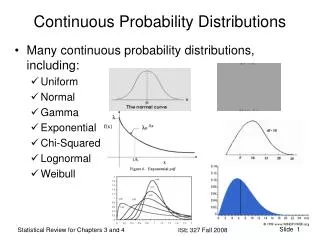
Continuous Probability Distributions

1. Continuous Probability Distributions • Continuous Random Variable • A random variable whose space (set of possible values) is an entire interval of numbers • Probability Density Function (or pdf) • The pdf, denoted f( x ), describes the distribution of probability across the set of possible values. • The probability that the random variable X takes on a value between a and b is equal to the area under f( x ) between a and b.

2. Probability Density Function • The pdf of a continuous random variable X has the following properties: • f( x ) ≥ 0, for every x  S • -∞∞ f( x ) dx = 1 • P( x  A ) = A f( x ) dx

3. Probability Density Function • So we have that: • P( a < x < b ) = ab f( x ) dx • P( X = a ) = aa f( x ) dx = 0 • P( a ≤ x ≤ b ) = P( a < x < b )

4. Histogram • A “connected” bar plot with bar height proportional to the frequency of the associated class. • Can be very useful for estimating a pdf. • Discrete Data • Each distinct outcome is marked on horizontal axis. • Bar is plotted atop each distinct outcome with bar height equal to frequency or relative frequency or that outcome.

5. Histogram • Continuous Data • Construct a frequency table • Partition data into classes and tabulate the frequency for each class. • Use frequency table to plot histogram • Mark class boundaries on horizontal axis and plot a bar on top of each class with height equal to the frequency or relative frequency of data in that class.

6. Cumulative Distribution Function • Called the cdf or distribution function • The cdf of a continuous random variable X is given by: F( x ) = P( X ≤ x ) = -∞x f( t ) dt • Consider that • P( a < X < b) = P( a ≤ x ≤ b ) = F( b ) – F( a ) • P( X > a ) = 1 – P( X ≤ a ) = 1 – F( a )

7. Cumulative Distribution Function • Using the fundamental theorem of calculus, it can be shown that:

8. Percentile • Let p be a number between 0 and 1, and let X be a continuous random variable with pdf f( x ) and cdf f( x ). • The 100·pth percentile is the number such that F( pp )=p. • Solve the following equation for pp:

9. Mathematical Expectation • The mathematical expectation of a continuous random variable X with pdf f( x ) is: m = E[ X ] = -∞∞x f( x ) dx • E[ X ] is also called the mean or expected value of X

10. Variance • The variance of a continuous random variable X with pdf f( x ) is: s2 = E[ ( X – m )2 ] = -∞∞( x – m )2 f( x ) dx = E[ X2 ] – (E[ X ])2 • measure of spread in f( x )

11. Expected Value of a Function • The expected value of the function h( x ) of a continuous random variable X with pdf f( x ) is: m = E[ h( X ) ] = -∞∞h( x ) f( x ) dx • Note that E[ h( X ) ] might not exist.

12. Continuous Uniform Distribution • Uniformly distributes the probability across the sample space. • If X is a continuous random variable on the interval [a,b], then • The pdf of X is: f( x ) = 1 / ( b – a ), for a ≤ x ≤ b

13. Continuous Uniform Distribution • If X is a continuous random variable on the interval [a,b], then • The cdf of X is: F( x ) = ( x – a ) / ( b – a ), for a ≤ x ≤ b • The mean and variance of X are: m = E[ X ] = ( a + b ) / 2 s2 = ( b – a )2 / 12

14. Exponential Distribution • Can be used to describe the waiting time between successive events in a Poisson process with mean l • If X is an exponential random variable from a Poisson process with mean l, then • The pdf of X is: f( x ) = le-lx, for x ≥ 0

15. Exponential Distribution • If X is an exponential random variable from a Poisson process with mean l, then • The cdf of X is: F( x ) = P ( X ≤ x ) = 1 - e-lx, for x ≥ 0 • So P ( X > x ) = 1 – F ( x ) = e-lx • The mean and variance of X are: m = 1/l s2 = 1/l2

16. Exponential Distribution • Memoryless Property • P( X > k + j | X > k ) = P( X > j ) • Percentiles of an Exponential • The pth percentile of an exponential random variable with mean 1/l is: pp = -1/l ln( 1 – p )

17. Normal Distribution • Commonly occurring distribution in nature and experimental settings. • symmetric, bell-shaped • A normal random variable X with mean m and variance s2 • is denoted: X ~ N( m, s2 ) • has pdf:

18. Standard Normal Distribution • A standard normal random variable is denoted Z and has distribution Z ~ N( 0, 1 ). • The pdf and cdf of a standard normal random variable are denoted f( z ) and F( z ) respectively. • Table A.3 contains probability values associated with F( z ). • Note that F( z ) = 1 - F( -z )

19. Standard Normal Distribution • za Notation • The value of Z that has a probability to its right is denoted za, so P( Z > za ) = a. by symmetry, P( Z < -za ) = P( Z > za ) = a • Percentile pp = z1-p

20. Non-Standard Normal Distribution • Any normal random variable X ~ N( m, s2 ) can be “standardized” into a Z by: Z = ( x – m ) / s • Percentile pp = m + z1-ps

21. Normal Approximation of Discrete Distributions • Many discrete random variables can be approximated by the normal distribution • A continuity correction of ±½ is required when estimating a discrete probability with the normal distribution

22. Normal Approximation of the Binomial Distribution • Let X be a binomial random variable with sample size n and probability of success p. If the sample size is sufficient ( np ≥ 5 and nq ≥ 5 ), then X can be approximated by a normal distribution with the same mean m=np and variance s2=npq. X ~ B( n, p )  N( np, npq ) PDF for Graphs: Binomial n=15, Binomial n=50, Binomial p=0.25

26. Normal Approximation of the Poisson Distribution • Let X be a Poisson random variable with sufficiently large mean l, then X can be approximated by a normal distribution with the same mean m=s2=npq. X ~ P( l )  N( l, l ) PDF for Graphs: Poisson ( l = 1, 5, 10, 15 )

28. Empirical Rule For data that is approximately normal in distribution (bell-shaped), • 68% of data values fall within 1 standard deviation of the mean, • 95.4% of data values fall within 2 standard deviation of the mean, • 99.7% of data values fall within 3 standard deviation of the mean,

29. 0.1% The Empirical Rule (applies to bell-shaped distributions) 99.7% of data are within 3 standard deviations of the mean 95% within 2 standard deviations 68% within 1 standard deviation 34% 34% 2.4% 2.4% 0.1% 13.5% 13.5% x - 3s x - 2s x - s x x+s x+2s x+3s

30. Identifying Unusual Observations • Range Rule of Thumb: • Empirical rule says 95% of observations should fall within 2s of the mean. Observations outside of m±2s are considered unusual. • Probability Approach: • The probability of the observed outcome or more extreme can be useful for identifying unusual observations. For example, if X is the observed outcome: • X is unusually high if P(x or more) is less than 0.05 • X is unusually low if P(x or less) is more than 0.05

31. Probability Plots • A probability plot can be useful for comparing the distribution of one sample data set to another. • If both data sets have the same sample size, then plot the order statistics from each sample against each other in a scatter plot. • Otherwise, plot order statistics from the smaller sample against corresponding sample percentiles from the other sample. • Note: The ith smallest observation is taken to be the (100*(i-½)/n)th sample percentile.

32. Measures of Relative Position • Percentile • The kth percentile (Pk) separates the bottom k% of data from the top (100-k)% of data. • The location of Pk in the order statistics is:

33. Interpretation of Probability Plots • Probability plot for comparing 2 sample data sets: • A straight line with slope 1 and y-intercept 0 indicates identical sample distributions. • A slope greater than 1 indicates that x is less variable than y. • A slope less than 1 indicates that x is more variable than y. • A y-intercept different from 0 indicates that the two samples have a different mean.

34. Probability Plots • A probability plot can be useful for comparing the distribution of sample data to a specified probability distribution. • Order statistics (or sample percentiles) of the sample are plotted against the corresponding percentiles of the probability distribution of interest. • Called the “Normal Probability Plot” when sample data is compared to normal percentiles.

35. Simulating Data from a Continuous Probability Distribution • Theorem • Let Y be U(0,1), a continuous uniform random variable on the interval (0,1). Let F( x ) have the properties of a cdf, then X = F -1( Y ) is a continuous random variable with cdf F( x ). • So, random data can be generate from any cdf that has an inverse function by generating random U(0,1) data and transforming it into F( x ) data.