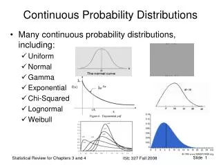
Continuous Probability Distributions
Continuous Probability Distributions. Continuous Random Variables and Probability Distributions. Random Variable: Y Cumulative Distribution Function (CDF): F ( y )=P( Y ≤ y ) Probability Density Function (pdf): f ( y )=d F ( y )/d y Rules governing continuous distributions:


Continuous Probability Distributions
E N D
Presentation Transcript
Continuous Random Variables and Probability Distributions • Random Variable: Y • Cumulative Distribution Function (CDF): F(y)=P(Y≤y) • Probability Density Function (pdf): f(y)=dF(y)/dy • Rules governing continuous distributions: • f(y) ≥ 0 y • P(a≤Y≤b) = F(b)-F(a) = • P(Y=a) = 0 a
Example – Cost/Benefit Analysis of Sprewell-Bluff Project (I) • Subjective Analysis of Annual Benefits/Costs of Project (U.S. Army Corps of Engineers assessments) • Y = Actual Benefit is Random Variable taken from a triangular distribution with 3 parameters: • A=Lower Bound (Pessimistic Outcome) • B=Peak (Most Likely Outcome) • C=Upper Bound (Optimistic Outcome) • 6 Benefit Variables • 3 Cost Variables Source: B.W. Taylor, R.M. North(1976). “The Measurement of Uncertainty in Public Water Resource Development,” American Journal of Agricultural Economics, Vol. 58, #4, Pt.1, pp.636-643
Example – Cost/Benefit Analysis of Sprewell-Bluff Project (II) ($1000s, rounded)
Example – Cost/Benefit Analysis of Sprewell-Bluff Project (III)(Flood Control, in $100K) Triangular Distribution with: lower bound=8.5 Peak=12.0 upper bound=15.0 Choose k area under density curve is 1: Area below 12.0 is: 0.5((12.0-8.5)k) = 1.75k Area above 12.0 is 0.5((15.0-12.0)k) = 1.50k Total Area is 3.25k k=1/3.25
Example – Cost/Benefit Analysis of Sprewell-Bluff Project (IV)(Flood Control)
Example – Cost/Benefit Analysis of Sprewell-Bluff Project (V)(Flood Control)
Example – Cost/Benefit Analysis of Sprewell-Bluff Project (VI) (Flood Control)
Example – Cost/Benefit Analysis of Sprewell-Bluff Project (VII) (Flood Control)
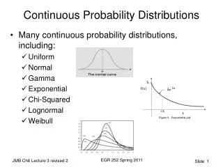
Uniform Distribution • Used to model random variables that tend to occur “evenly” over a range of values • Probability of any interval of values proportional to its width • Used to generate (simulate) random variables from virtually any distribution • Used as “non-informative prior” in many Bayesian analyses
Exponential Distribution • Right-Skewed distribution with maximum at y=0 • Random variable can only take on positive values • Used to model inter-arrival times/distances for a Poisson process
Gamma Function EXCEL Function: =EXP(GAMMALN(a))
Exponential/Poisson Connection • Consider a Poisson process with random variable X being the number of occurences of an event in a fixed time/space X(t)~Poisson(lt) • Let Y be the distance in time/space between two such events • Then if Y > y, no events have occurred in the space of y
Gamma Distribution • Family of Right-Skewed Distributions • Random Variable can take on positive values only • Used to model many biological and economic characteristics • Can take on many different shapes to match empirical data Obtaining Probabilities in EXCEL: To obtain: F(y)=P(Y≤y) Use Function: =GAMMADIST(y,a,b,1)
Gamma Distribution – Special Cases • Exponential Distribution – a=1 • Chi-Square Distribution – a=n/2, b=2 (n ≡ integer) • E(Y)=n V(Y)=2n • M(t)=(1-2t)-n/2 • Distribution is widely used for statistical inference • Notation: Chi-Square with n degrees of freedom:
Normal (Gaussian) Distribution • Bell-shaped distribution with tendency for individuals to clump around the group median/mean • Used to model many biological phenomena • Many estimators have approximate normal sampling distributions (see Central Limit Theorem) Obtaining Probabilities in EXCEL: To obtain: F(y)=P(Y≤y) Use Function: =NORMDIST(y,m,s,1)
Beta Distribution • Used to model probabilities (can be generalized to any finite, positive range) • Parameters allow a wide range of shapes to model empirical data Obtaining Probabilities in EXCEL: To obtain: F(y)=P(Y≤y) Use Function: =BETADIST(y,a,b)
Weibull Distribution Note: The EXCEL function WEIBULL(y,a*,b*) uses parameterization: a*=b, b*=ab
Lognormal Distribution Obtaining Probabilities in EXCEL: To obtain: F(y)=P(Y≤y) Use Function: =LOGNORMDIST(y,m,s)