Continuous Probability Distributions
Continuous Probability Distributions. Chapter 8. 0. 1/3. 1/2. 1. 2/3. 8.2 Continuous Probability Distributions. A continuous random variable has an uncountably infinite number of values in the interval (a,b).


Continuous Probability Distributions
E N D
Presentation Transcript
Continuous Probability Distributions Chapter 8
0 1/3 1/2 1 2/3 8.2 Continuous Probability Distributions • A continuous random variable has an uncountably infinite number of values in the interval (a,b). • The probability that a continuous variable X will assume any particular value is zero. Why? The probability of each value 1/4 + 1/4 + 1/4 + 1/4 = 1 1/3 + 1/3 + 1/3 = 1 1/2 + 1/2 = 1
0 1/3 1/2 1 2/3 8.2 Continuous Probability Distributions As the number of values increases the probability of each value decreases. This is so because the sum of all the probabilities remains 1. When the number of values approaches infinity (because X is continuous) the probability of each value approaches 0. The probability of each value 1/4 + 1/4 + 1/4 + 1/4 = 1 1/3 + 1/3 + 1/3 = 1 1/2 + 1/2 = 1
Area = 1 x1 x2 Probability Density Function • To calculate probabilities we define a probability density function f(x). • The density function satisfies the following conditions • f(x) is non-negative, • The total area under the curve representing f(x) equals 1. P(x1<=X<=x2) • The probability that X falls between x1 and x2 is found by calculating the area under the graph of f(x) between x1 and x2.
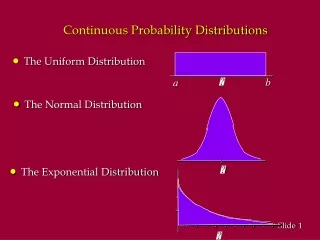
Uniform Distribution • A random variable X is said to be uniformly distributed if its density function is • The expected value and the variance are
Uniform Distribution • Example 8.1 • The daily sale of gasoline is uniformly distributed between 2,000 and 5,000 gallons. Find the probability that sales are: • Between 2,500 and 3,500 gallons • More than 4,000 gallons • Exactly 2,500 gallons f(x) = 1/(5000-2000) = 1/3000 for x: [2000,5000] P(2500£X£3000) = (3000-2500)(1/3000) = .1667 1/3000 x 2000 2500 3000 5000
Uniform Distribution • Example 8.1 • The daily sale of gasoline is uniformly distributed between 2,000 and 5,000 gallons. Find the probability that sales are: • Between 2,500 and 3,500 gallons • More than 4,000 gallons • Exactly 2,500 gallons f(x) = 1/(5000-2000) = 1/3000 for x: [2000,5000] P(X³4000) = (5000-4000)(1/3000) = .333 1/3000 x 2000 4000 5000
Uniform Distribution • Example 8.1 • The daily sale of gasoline is uniformly distributed between 2,000 and 5,000 gallons. Find the probability that sales are: • Between 2,500 and 3,500 gallons • More than 4,000 gallons • Exactly 2,500 gallons f(x) = 1/(5000-2000) = 1/3000 for x: [2000,5000] P(X=2500) = (2500-2500)(1/3000) = 0 1/3000 x 2000 2500 5000
8.3 Normal Distribution • This is the most important continuous distribution. • Many distributions can be approximated by a normal distribution. • The normal distribution is the cornerstone distribution of statistical inference.
Normal Distribution • A random variable X with mean m and variance s2is normally distributed if its probability density function is given by
The Shape of the Normal Distribution The normal distribution is bell shaped, and symmetrical around m. m 90 110 Why symmetrical? Let m = 100. Suppose x = 110. Now suppose x = 90
The effects of m and s The effects of m and s How does the standard deviation affect the shape of f(x)? s= 2 s =3 s =4 How does the expected value affect the location of f(x)? m = 10 m = 11 m = 12
Finding Normal Probabilities • Two facts help calculate normal probabilities: • The normal distribution is symmetrical. • Any normal distribution can be transformed into a specific normal distribution called… • “STANDARD NORMAL DISTRIBUTION” Example The amount of time it takes to assemble a computer is normally distributed, with a mean of 50 minutes and a standard deviation of 10 minutes. What is the probability that a computer is assembled in a time between 45 and 60 minutes?
Finding Normal Probabilities • Solution • If X denotes the assembly time of a computer, we seek the probability P(45<X<60). • This probability can be calculated by creating a new normal variable the standard normal variable. Every normal variable with some m and s, can be transformed into this Z. Therefore, once probabilities for Z are calculated, probabilities of any normal variable can be found. V(Z) = s2 = 1 E(Z) = m = 0
Finding Normal Probabilities • Example - continued - m 45 - 50 X 60 - 50 P(45<X<60) = P( < < ) s 10 10 = P(-0.5 < Z < 1) To complete the calculation we need to compute the probability under the standard normal distribution
P(0<Z<z0) Using the Standard Normal Table Standard normal probabilities have been calculated and are provided in a table . The tabulated probabilities correspond to the area between Z=0 and some Z = z0 >0 Z = z0 Z = 0
- m 45 - 50 X 60 - 50 P(45<X<60) = P( < < ) s 10 10 z0 = 1 z0 = -.5 Finding Normal Probabilities • Example - continued = P(-.5 < Z < 1) We need to find the shaded area
- m 45 - 50 X 60 - 50 P(45<X<60) = P( < < ) s 10 10 z0 = 1 z0 =-.5 Finding Normal Probabilities • Example - continued = P(-.5<Z<1) = P(-.5<Z<0)+ P(0<Z<1) P(0<Z<1 .3413 z=0
Finding Normal Probabilities • The symmetry of the normal distribution makes it possible to calculate probabilities for negative values of Z using the table as follows: -z0 +z0 0 P(-z0<Z<0) = P(0<Z<z0)
Finding Normal Probabilities • Example - continued .3413 .1915 -.5 .5
.1915 .1915 .1915 .1915 Finding Normal Probabilities • Example - continued .3413 1.0 -.5 .5 P(-.5<Z<1) = P(-.5<Z<0)+ P(0<Z<1) = .1915 + .3413 = .5328
0% 10% Finding Normal Probabilities • Example 8.2 • The rate of return (X) on an investment is normally distributed with mean of 10% and standard deviation of (i) 5%, (ii) 10%. • What is the probability of losing money? X 0 - 10 5 .4772 (i) P(X< 0 ) = P(Z< ) = P(Z< - 2) Z 2 -2 0 =P(Z>2) = 0.5 - P(0<Z<2) = 0.5 - .4772 = .0228
0% 10% 1 Find Normal Probabilities Finding Normal Probabilities • Example 8.2 • The rate of return (X) on an investment is normally distributed with mean of 10% and standard deviation of (i) 5%, (ii) 10%. • What is the probability of losing money? X 0 - 10 10 .3413 (ii) P(X< 0 ) = P(Z< ) Z -1 = P(Z< - 1) = P(Z>1) = 0.5 - P(0<Z<1) = 0.5 - .3413 = .1587
Finding Values of Z • Sometimes we need to find the value of Z for a given probability • We use the notation zA to express a Z value for which P(Z > zA) = A A zA
0.05 Finding Values of Z • Example 8.3 & 8.4 • Determine z exceeded by 5% of the population • Determine z such that 5% of the population is below • Solution z.05is defined as the z value for which the area on its right under the standard normal curve is .05. 0.45 0.05 1.645 Z0.05 -Z0.05 0
Exponential Distribution • The exponential distribution can be used to model • the length of time between telephone calls • the length of time between arrivals at a service station • the life-time of electronic components. • When the number of occurrences of an event follows the Poisson distribution, the time between occurrences follows the exponential distribution.
Exponential Distribution A random variable is exponentially distributed if its probability density function is given byf(x) = le-lx, x>=0. lis the distribution parameter (l>0). E(X) = 1/l V(X) = (1/l)2
f(x) = 2e-2x f(x) = 1e-1x f(x) = .5e-.5x 0 1 2 3 4 5 Exponential distribution for l = .5, 1, 2 P(a<x<b) = e-la - e-lb a b
Exponential Distribution • Finding exponential probabilities is relatively easy: • P(X > a) = e–la. • P(X < a) = 1 – e –la • P(a1 < X < a2) = e – l(a1) – e – l(a2)
Exponential Distribution • Example 8.5 • The lifetime of an alkaline battery is exponentially distributed with l = .05 per hour. • What is the mean and standard deviation of the battery’s lifetime? • Find the following probabilities: • The battery will last between 10 and 15 hours. • The battery will last for more than 20 hours?
Exponential Distribution • Solution • The mean = standard deviation = 1/l = 1/.05 = 20 hours. • Let X denote the lifetime. • P(10<X<15) = e-.05(10) – e-.05(15) = .1341 • P(X > 20) = e-.05(20) = .3679
Exponential Distribution • Example 8.6 • The service rate at a supermarket checkout is 6 customers per hour. • If the service time is exponential, find the following probabilities: • A service is completed in 5 minutes, • A customer leaves the counter more than 10 minutes after arriving • A service is completed between 5 and 8 minutes.
Compute Exponential probabilities Exponential Distribution • Solution • A service rate of 6 per hour = A service rate of .1 per minute (l = .1/minute). • P(X < 5) = 1-e-lx = 1 – e-.1(5) = .3935 • P(X >10) = e-lx = e-.1(10) = .3679 • P(5 < X < 8) = e-.1(5) – e-.1(8) = .1572
8.5 Other Continuous Distribution • Three new continuous distributions: • Student t distribution • Chi-squared distribution • F distribution
The Student t Distribution • The Student t density function n is the parameter of the student t distribution E(t) = 0 V(t) = n/(n – 2) (for n > 2)
The Student t Distribution n = 3 n = 10
Determining Student t Values • The student t distribution is used extensively in statistical inference. • Thus, it is important to determine values of tA associated with a given number of degrees of freedom. • We can do this using • t tables • Excel • Minitab
A A = .05 = .05 -tA Using the t Table t t t t • The table provides the t values (tA) for which P(tn > tA) = A The t distribution is symmetrical around 0 tA =-1.812 =1.812 t.100 t.05 t.025 t.01 t.005
The Chi – Squared Distribution • The Chi – Squared density function: • The parameter n is the number of degrees of freedom.
Determining Chi-Squared Values • Chi squared values can be found from the chi squared table, from Excel, or from Minitab. • The c2-table entries are the c2 values of the right hand tail probability (A), for which P(c2n > c2A) = A. A c2A
A c2A Using the Chi-Squared Table To find c2 for which P(c2n<c2)=.01, lookup the column labeledc21-.01 or c2.99 =.05 A =.99 c2.05 c2.995 c2.990 c2.05 c2.010 c2.005
! ! ! The F Distribution • The density function of the F distribution:n1 and n2 are the numerator and denominator degrees of freedom.
The F Distribution • This density function generates a rich family of distributions, depending on the values of n1 and n2 n1 = 5, n2 = 10 n1 = 50, n2 = 10 n1 = 5, n2 = 10 n1 = 5, n2 = 1
Determining Values of F • The values of the F variable can be found in the F table, Excel, or from Minitab. • The entries in the table are the values of the F variable of the right hand tail probability (A), for which P(Fn1,n2>FA) = A.