Continuous Probability Distributions
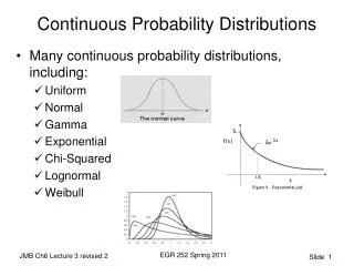
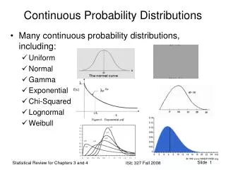
Continuous Probability Distributions. The Normal Distribution. Data Distribution. Random. Left Skew. Right Skew. Standard Normal Distribution. The Classic Bell-Shaped curve is symmetric, with mean = median = mode = midpoint. 50% of values less than the mean and 50% greater than the mean.


Continuous Probability Distributions
E N D
Presentation Transcript
Continuous Probability Distributions The Normal Distribution
Data Distribution Random Left Skew Right Skew
Standard Normal Distribution The Classic Bell-Shaped curve is symmetric, with mean = median = mode = midpoint 50% of values less than the mean and 50% greater than the mean
This is a bell shaped curve with different centers and spreads depending on and The Normal Distribution:as mathematical function (pdf) Note constants: =3.14159 e=2.71828
The Normal PDF It’s a probability function, so no matter what the values of and , must integrate to 1!
Normal distribution is defined by its mean and standard dev. E(X)= = Var(X)=2 = Standard Deviation(X)=
Three Sigma Rule • Area between - and + is about 68% • Area between -2 and +2 is about 95% • Area between -3 and +3 is about 99.7% • Almost all values fall within 3 standard deviations.
68% of the data 95% of the data 99.7% of the data Three Sigma Rule
Normal Probability Distribution • The distribution is symmetric, with a mean of zero and standard deviation of 1. • The probability of a score between 0 and 1 is the same as the probability of a score between 0 and –1: both are .34.
Standard Normal Distribution (Z) All normal distributions can be converted into the standard normal curve by subtracting the mean and dividing by the standard deviation:
Why Standardize ... ? • A teacher marks a test students results (out of 60 points): • 20, 15, 26, 32, 18, 28, 35, 14, 26, 22, 17 • Standardize all the scores with Mean 23, and the Standard Deviation 6.6. • -0.45, -1.21, 0.45, 1.36, -0.76, 0.76, 1.82, -1.36, 0.45, -0.15, -0.91 • only fail students 1 standard deviation below the mean.
Comparing X and Z units 100 200 X ( = 100, = 50) 0 2.0 Z ( = 0, = 1)
Calculating Normal Distribution • Find Mean and Standard Deviation • Find Standardized Random Variable • Use Normal Distribution Table (A7) • Ф(-z) = 1 – Ф(z)
Problem 1 Let X be normal with Mean 80 and Variance 9. Find P(X > 83), (X < 81), P(X < 80), and P(78 < X < 83).
Problem 2 Let X be normal with Mean 120 and Variance 16. Find P(X < 126), (X > 116), and P(125 < X < 130).
Calculating Normal Distribution • Find Mean and Standard Deviation • Find Standardized Random Variable • If Ф(z) = % given, Use Normal Distribution Table (A8) • D(z) = Ф(z) – Ф(-z)
Problem 3 Let X be normal with Mean 14 and Variance 4. Determine c such that P(X ≤ c) = 95%, P(X ≤ c) = 5%, and P(X ≤ c) = 99.5%
Problem 4 Let X be normal with Mean 4.2 and Variance 4. Determine c such that P(X ≤ c) = 90%.
Calculating Normal Distribution • X < Mean = 0.5 – Z • X > Mean = 0.5 + Z • X = Mean = 0.5 • X = Normal Random Variable
Example • What’s the probability of getting a math SAT score of 575 or less, =500 and =50? • i.e., A score of 575 is 1.5 standard deviations above the mean Look up Z= 1.5 in standard normal chart = .9332
Z=1.51 Z=1.51 Looking up probabilities in the standard normal table
The “probnorm(Z)” function gives you the probability from negative infinity to Z (here 1.5) in a standard normal curve. The “probit(p)” function gives you the Z-value that corresponds to a left-tail area of p (here .93) from a standard normal curve. The probit function is also known as the inverse standard normal function. Normal probabilities in SAS data _null_; theArea=probnorm(1.5); put theArea; run; 0.9331927987 And if you wanted to go the other direction (i.e., from the area to the Z score (called the so-called “Probit” function data _null_; theZValue=probit(.93); put theZValue; run; 1.4757910282
Practice problem If birth weights in a population are normally distributed with a mean of 109 oz and a standard deviation of 13 oz, • What is the chance of obtaining a birth weight of 141 oz or heavier when sampling birth records at random? • What is the chance of obtaining a birth weight of 120 or lighter?
Answer • What is the chance of obtaining a birth weight of 141 oz or heavier when sampling birth records at random? From the chart or SAS Z of 2.46 corresponds to a right tail (greater than) area of: P(Z≥2.46) = 1-(.9931)= .0069 or .69 %
Answer b. What is the chance of obtaining a birth weight of 120 or lighter? From the chart or SAS Z of .85 corresponds to a left tail area of: P(Z≤.85) = .8023= 80.23%
Probit function: the inverse (area)= Z: gives the Z-value that goes with the probability you want For example, recall SAT math scores example. What’s the score that corresponds to the 90th percentile? In Table, find the Z-value that corresponds to area of .90 Z= 1.28 Or use SAS data _null_; theZValue=probit(.90); put theZValue; run; 1.2815515655 If Z=1.28, convert back to raw SAT score 1.28 = X – 500 =1.28 (50) X=1.28(50) + 500 = 564 (1.28 standard deviations above the mean!) `
Are my data “normal”? • Not all continuous random variables are normally distributed!! • It is important to evaluate how well the data are approximated by a normal distribution
Are my data normally distributed? • Look at the histogram! Does it appear bell shaped? • Compute descriptive summary measures—are mean, median, and mode similar? • Do 2/3 of observations lie within 1 std dev of the mean? Do 95% of observations lie within 2 std dev of the mean? • Look at a normal probability plot—is it approximately linear? • Run tests of normality (such as Kolmogorov-Smirnov). But, be cautious, highly influenced by sample size!
Data from our class… Median = 6 Mean = 7.1 Mode = 0 SD = 6.8 Range = 0 to 24 (= 3.5 σ)
Data from our class… Median = 5 Mean = 5.4 Mode = none SD = 1.8 Range = 2 to 9 (~ 4 σ)
Data from our class… Median = 3 Mean = 3.4 Mode = 3 SD = 2.5 Range = 0 to 12 (~ 5 σ)
Data from our class… Median = 7:00 Mean = 7:04 Mode = 7:00 SD = :55 Range = 5:30 to 9:00 (~4 σ)
13.9 0.3 Data from our class… 7.1 +/- 6.8 = 0.3 – 13.9
Data from our class… 7.1 +/- 2*6.8 = 0 – 20.7
Data from our class… 7.1 +/- 3*6.8 = 0 – 27.5
3.6 7.2 Data from our class… 5.4 +/- 1.8 = 3.6 – 7.2
9.0 1.8 Data from our class… 5.4 +/- 2*1.8 = 1.8 – 9.0
10 0 Data from our class… 5.4 +/- 3*1.8 = 0– 10
0.9 5.9 Data from our class… 3.4 +/- 2.5= 0.9 – 7.9
0 8.4 Data from our class… 3.4 +/- 2*2.5= 0 – 8.4
0 10.9 Data from our class… 3.4 +/- 3*2.5= 0 – 10.9
6:09 7:59 Data from our class… 7:04+/- 0:55 = 6:09 – 7:59
5:14 8:54 Data from our class… 7:04+/- 2*0:55 = 5:14 – 8:54
4:19 9:49 Data from our class… 7:04+/- 2*0:55 = 4:19 – 9:49
The Normal Probability Plot • Normal probability plot • Order the data. • Find corresponding standardized normal quantile values: • Plot the observed data values against normal quantile values. • Evaluate the plot for evidence of linearity.
Normal probability plot coffee… Right-Skewed! (concave up)
Normal probability plot love of writing… Neither right-skewed or left-skewed, but big gap at 6.